Introduction to Regression Procedures: Multivariate Tests

Introduction to Regression Procedures

Multivariate Tests

Multivariate hypotheses involve several dependent variables in the form

$\text{[math]}$

where $\text{[math]}$ is a linear function on the regressor side, $\text{[math]}$ is a matrix of parameters, $\text{[math]}$ is a linear function on the dependent side, and $\text{[math]}$ is a matrix of constants. The special case (handled by PROC REG) in which the constants are the same for each dependent variable is expressed as

$\text{[math]}$

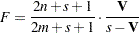
where $\text{[math]}$ is a column vector of constants and $\text{[math]}$ is a row vector of 1s. The special case in which the constants are 0 is then

$\text{[math]}$

These multivariate tests are covered in detail in Morrison (1976), Timm (1975), Mardia, Kent, and Bibby (1979), Bock (1975), and other works cited in Chapter 9, Introduction to Multivariate Procedures.

Notice that in contrast to the tests discussed in the preceding section, $\text{[math]}$ here is a matrix of parameter estimates. Suppose that the matrix of estimates is denoted as $\text{[math]}$ . To test the multivariate hypothesis, construct two matrices, $\text{[math]}$ and $\text{[math]}$ , that correspond to the numerator and denominator of a univariate $\text{[math]}$ test:

	$\text{[math]}$	$\text{[math]}$
	$\text{[math]}$	$\text{[math]}$

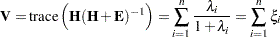
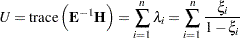
Four test statistics, based on the eigenvalues of $\text{[math]}$ or $\text{[math]}$ , are formed. Let $\text{[math]}$ be the ordered eigenvalues of $\text{[math]}$ (if the inverse exists), and let $\text{[math]}$ be the ordered eigenvalues of $\text{[math]}$ . It happens that $\text{[math]}$ and $\text{[math]}$ , and it turns out that $\text{[math]}$ is the $\text{[math]}$ th canonical correlation.

Let $\text{[math]}$ be the rank of $\text{[math]}$ , which is less than or equal to the number of columns of $\text{[math]}$ . Let $\text{[math]}$ be the rank of $\text{[math]}$ . Let $\text{[math]}$ be the error degrees of freedom and $\text{[math]}$ . Let $\text{[math]}$ , and let $\text{[math]}$ . Then the following statistics test the multivariate hypothesis in various ways, and their p-values can be approximated by $\text{[math]}$ distributions. Note that in the special case that the rank of $\text{[math]}$ is 1, all of these $\text{[math]}$ statistics will be the same and the corresponding p-values will in fact be exact, since in this case the hypothesis is really univariate.

Wilks’ Lambda

$\text{[math]}$

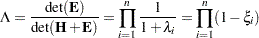then

$\text{[math]}$

is approximately $\text{[math]}$ distributed, where

	$\text{[math]}$	$\text{[math]}$
	$\text{[math]}$	$\text{[math]}$
	$\text{[math]}$	$\text{[math]}$

The degrees of freedom are $\text{[math]}$ and $\text{[math]}$ . The distribution is exact if $\text{[math]}$ . (See Rao 1973, p. 556.)

Pillai’s Trace

$\text{[math]}$

then

$\text{[math]}$

is approximately $\text{[math]}$ distributed with $\text{[math]}$ and $\text{[math]}$ degrees of freedom.

Hotelling-Lawley Trace

$\text{[math]}$

then for $\text{[math]}$

$\text{[math]}$

is approximately $\text{[math]}$ distributed with $\text{[math]}$ and $\text{[math]}$ degrees of freedom, where $\text{[math]}$ and $\text{[math]}$ ; while for $\text{[math]}$

$\text{[math]}$

is approximately $\text{[math]}$ with $\text{[math]}$ and $\text{[math]}$ degrees of freedom.

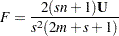
Roy’s Maximum Root

If $\text{[math]}$ , then

$\text{[math]}$

where $\text{[math]}$ is an upper bound on $\text{[math]}$ that yields a lower bound on the significance level. Degrees of freedom are $\text{[math]}$ for the numerator and $\text{[math]}$ for the denominator.

Tables of critical values for these statistics are found in Pillai (1960).

Exact Multivariate Tests

Beginning with SAS 9, if you specify the MSTAT=EXACT option in the appropriate statement, p-values for three of the four tests are computed exactly (Wilks’ lambda, the Hotelling-Lawley trace, and Roy’s greatest root), and the p-values for the fourth (Pillai’s trace) are based on an $\text{[math]}$ approximation that is more accurate (but occasionally slightly more liberal) than the default. The exact p-values for Roy’s greatest root benefit the most, since in this case the $\text{[math]}$ approximation provides only a lower bound for the $\text{[math]}$ -value. If you use the $\text{[math]}$ -based $\text{[math]}$ -value for this test in the usual way, declaring a test significant if $\text{[math]}$ , then your decisions might be very liberal. For example, instead of the nominal 5% Type I error rate, such a procedure can easily have an actual Type I error rate in excess of 30%. By contrast, basing such a procedure on the exact p-values will result in the appropriate 5% Type I error rate, under the usual regression assumptions.

The MSTAT=EXACT option is supported in the ANOVA, CANCORR, CANDISC, GLM, and REG procedures.

The exact $\text{[math]}$ -values are based on the following sources:

Wilks’ lambda: Lee (1972), Davis (1979)
Pillai’s trace: Muller (1998)
Hotelling-Lawley trace: Davis (1970), Davis (1980)
Roy’s greatest root: Davis (1972), Pillai and Flury (1984)

Note that, although the MSTAT=EXACT $\text{[math]}$ -value for Pillai’s trace is still approximate, it has "substantially greater accuracy" than the default approximation (Muller 1998).

Since most of the MSTAT=EXACT $\text{[math]}$ -values are not based on the $\text{[math]}$ distribution, the columns in the multivariate tests table corresponding to this approximation—in particular, the $\text{[math]}$ value and the numerator and denominator degrees of freedom—are no longer displayed, and the column containing the $\text{[math]}$ -values is labeled “P Value” instead of "Pr > F." Suppose, for example, you use the following PROC ANOVA statements to perform a multivariate analysis of an archaeological data set:

data Skulls;
   input Loc $20. Basal Occ Max;
   datalines;
Minas Graes, Brazil  2.068 2.070 1.580
Minas Graes, Brazil  2.068 2.074 1.602
Minas Graes, Brazil  2.090 2.090 1.613
Minas Graes, Brazil  2.097 2.093 1.613
Minas Graes, Brazil  2.117 2.125 1.663
Minas Graes, Brazil  2.140 2.146 1.681
Matto Grosso, Brazil 2.045 2.054 1.580
Matto Grosso, Brazil 2.076 2.088 1.602
Matto Grosso, Brazil 2.090 2.093 1.643
Matto Grosso, Brazil 2.111 2.114 1.643
Santa Cruz, Bolivia  2.093 2.098 1.653
Santa Cruz, Bolivia  2.100 2.106 1.623
Santa Cruz, Bolivia  2.104 2.101 1.653
;

proc anova data=Skulls;
   class Loc;
   model Basal Occ Max = Loc / nouni;
   manova h=Loc;
   ods select MultStat;
run;

The default multivariate tests, based on the $\text{[math]}$ approximations, are shown in Figure 4.5.

Figure 4.5 Default Multivariate Tests

The ANOVA Procedure

Multivariate Analysis of Variance

MANOVA Test Criteria and F Approximations for the Hypothesis of No Overall Loc Effect H = Anova SSCP Matrix for Loc E = Error SSCP Matrix S=2 M=0 N=3
Statistic	Value	F Value	Num DF	Den DF	Pr > F
Wilks' Lambda	0.60143661	0.77	6	16	0.6032
Pillai's Trace	0.44702843	0.86	6	18	0.5397
Hotelling-Lawley Trace	0.58210348	0.75	6	9.0909	0.6272
Roy's Greatest Root	0.35530890	1.07	3	9	0.4109
NOTE: F Statistic for Roy's Greatest Root is an upper bound.
NOTE: F Statistic for Wilks' Lambda is exact.

If you specify MSTAT=EXACT in the MANOVA statement, as in the following statements, then the displayed output is the much simpler table shown in Figure 4.6.

proc anova data=Skulls;
   class Loc;
   model Basal Occ Max = Loc / nouni;
   manova h=Loc / mstat=exact;
   ods select MultStat;
run;

Figure 4.6 Multivariate Tests with MSTAT=EXACT

The ANOVA Procedure

Multivariate Analysis of Variance

MANOVA Tests for the Hypothesis of No Overall Loc Effect H = Anova SSCP Matrix for Loc E = Error SSCP Matrix S=2 M=0 N=3
Statistic	Value	P-Value
Wilks' Lambda	0.60143661	0.6032
Pillai's Trace	0.44702843	0.5521
Hotelling-Lawley Trace	0.58210348	0.6337
Roy's Greatest Root	0.35530890	0.7641

Notice that the $\text{[math]}$ -value for Roy’s greatest root is substantially larger in the new table, and correspondingly more in line with the $\text{[math]}$ -values for the other tests.

If you reference the underlying ODS output object for the table of multivariate statistics, it is important to note that its structure does not depend on the value of the MSTAT= specification. In particular, it always contains columns corresponding to both the default MSTAT=FAPPROX and the MSTAT=EXACT tests. Moreover, since the MSTAT=FAPPROX tests are relatively cheap to compute, the columns corresponding to them are always filled in, even though they are not displayed when you specify MSTAT=EXACT. On the other hand, for MSTAT=FAPPROX (which is the default), the column of exact $\text{[math]}$ -values contains missing values, and is not displayed.

Top of Page