| Introduction to Structural Equation Modeling with Latent Variables |
A Combined Measurement-Structural Model
To illustrate a more complex model, this example uses some well-known data from Haller and Butterworth (1960). Various models and analyses of these data are given by Duncan, Haller, and Portes (1968), Jöreskog and Sörbom (1988), and Loehlin (1987).
The study concerns the career aspirations of high school students and how these aspirations are affected by close friends. The data are collected from 442 seventeen-year-old boys in Michigan. There are 329 boys in the sample who named another boy in the sample as a best friend. The data from these 329 boys paired with the data from their best friends are analyzed.
The method of data collection introduces two statistical problems. First, restricting the analysis to boys whose best friends are in the original sample causes the reduced sample to be biased. Second, since the data from a given boy might appear in two or more observations, the observations are not independent. Therefore, any statistical conclusions should be considered tentative. It is difficult to accurately assess the effects of the dependence of the observations on the analysis, but it could be argued on intuitive grounds that since each observation has data from two boys and since it seems likely that many of the boys appear in the data set at least twice, the effective sample size might be as small as half of the reported 329 observations.
The correlation matrix, taken from Jöreskog and Sörbom (1988), is shown in the following DATA step:
title 'Peer Influences on Aspiration: Haller & Butterworth (1960)';
data aspire(type=corr);
   _type_='corr';
   input _name_ $ riq rpa rses roa rea fiq fpa fses foa fea;
   label riq='Respondent: Intelligence'
         rpa='Respondent: Parental Aspiration'
         rses='Respondent: Family SES'
         roa='Respondent: Occupational Aspiration'
         rea='Respondent: Educational Aspiration'
         fiq='Friend: Intelligence'
         fpa='Friend: Parental Aspiration'
         fses='Friend: Family SES'
         foa='Friend: Occupational Aspiration'
         fea='Friend: Educational Aspiration';
   datalines;
riq   1.      .      .      .      .      .       .      .      .      .
rpa   .1839  1.      .      .      .      .       .      .      .      .
rses  .2220  .0489  1.      .      .      .       .      .      .      .
roa   .4105  .2137  .3240  1.      .      .       .      .      .      .
rea   .4043  .2742  .4047  .6247  1.      .       .      .      .      .
fiq   .3355  .0782  .2302  .2995  .2863  1.       .      .      .      .
fpa   .1021  .1147  .0931  .0760  .0702  .2087   1.      .      .      .
fses  .1861  .0186  .2707  .2930  .2407  .2950  -.0438  1.      .      .
foa   .2598  .0839  .2786  .4216  .3275  .5007   .1988  .3607  1.      .
fea   .2903  .1124  .3054  .3269  .3669  .5191   .2784  .4105  .6404  1.
;
Career Aspiration: Analysis 1
The model analyzed by Jöreskog and Sörbom (1988) is displayed in the path diagram in Figure 17.35.
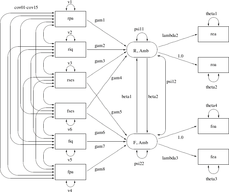
Two latent variables, R_Amb and F_Amb, represent the respondent’s level of ambition and his best friend’s level of ambition, respectively. The model states that the respondent’s ambition (R_Amb) is determined by his intelligence (riq) and socioeconomic status (rses), his perception of his parents’ aspiration for him (rpa), and his friend’s socioeconomic status (fses) and ambition (F_Amb). It is assumed that his friend’s intelligence (fiq) and parental aspiration (fpa) affect the respondent’s ambition only indirectly through the friend’s ambition (F_Amb). Ambition is indicated by the manifest variables of occupational (roa) and educational aspiration (rea), which are assumed to have uncorrelated residuals. The path coefficient from ambition to occupational aspiration is set to 1.0 to determine the scale of the ambition latent variable.
The path diagram shown in Figure 17.35 appears to be very complicated. Sometimes when researchers draw their path diagram with a lot of variables, they omit the covariances among exogenous variables for overall clarity. For example, the double-headed paths that represent cov01–cov15 in Figure 17.35 can be omitted. In addition, unconstrained variance and error variance parameters in the path diagram could be omitted without losing the pertinent information in the path diagram. For example, variance parameters v1–v6 and error variance parameters theta1–theta4 in Figure 17.35 detract from the main focus on the functional relationships of the model.
These omissions in the path diagram are in fact inconsequential when you transcribe them into the PATH model in PROC CALIS. The reason is that PROC CALIS employs several useful default parameterization rules that make the model specification process much easier and more intuitive. Here are the sets of default covariance structure parameters in the PATH modeling language:
variances for all exogenous (observed or latent) variables
error variances of all endogenous (observed or latent) variables
covariances among all exogenous (observed or latent, excluding error) variables
For example, these rules for setting default covariance structure parameters mean that the following sets of parameters in Figure 17.35 are optional in the path diagram representation and in the corresponding PATH model specification:
v1–v6
theta1–theta4, psi11, and psi22
cov01–cov15
Note that the double-headed path labeled with psi12, which is a covariance parameter among error terms for R_Amb and F_Amb, is not a default parameter. As a result, it must be represented in the path diagram and in the PATH model specification.
Another simplification is to omit the unconstrained parameter names in the path diagram. In the PATH model specification, an "unnamed" parameter is a free parameter by default—there is no need to give unique names to denote free parameters. With all the mentioned simplifications, you can depict your path diagram simply as the one in Figure 17.36.
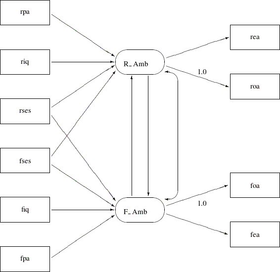
The simplified path diagram in Figure 17.36 is readily transcribed into the PATH model as shown in the following statements:
proc calis data=aspire nobs=329;
   path
      /* structural model of influences */
      R_Amb <--- rpa     ,
      R_Amb <--- riq     ,
      R_Amb <--- rses    ,
      R_Amb <--- fses    ,
      F_Amb <--- rses    ,
      F_Amb <--- fses    ,
      F_Amb <--- fiq     ,
      F_Amb <--- fpa     ,
      R_Amb <--- F_Amb   ,
      F_Amb <--- R_Amb   ,

      /* measurement model for aspiration */
      rea <---  R_Amb      ,
      roa <---  R_Amb  = 1.,
      foa <---  F_Amb  = 1.,
      fea <---  F_Amb    ;
   pcov
      R_Amb  F_Amb;
run;
Again, because you have 15 paths (single- or double- headed) in the path diagram, you expect that there are 15 entries in the PATH and the PCOV statements. Essentially, in this PATH model specification you specify all the functional relationships in the path diagram and the covariance of error terms for R_Amb and F_Amb.
Since this TYPE=CORR data set does not contain an observation with _TYPE_=N giving the sample size, it is necessary to specify the NOBS= option in the PROC CALIS statement.
The fit summary is displayed in Figure 17.37, and the estimation results are displayed in Figure 17.38.
The model fit chi-square value is 26.6972 ( =15,
=15,  =0.0313). From the hypothesis testing point of view, this result says that this is an extreme sample given the model is true; therefore, the model should be rejected. But in social and behavioral sciences, you rarely abandon a model purely on the ground of chi-square significance test. The main reason is that you might only need to find a model that is approximately true, but the hypothesis testing framework is for testing exact model representation in the population. To determine whether a model is good or bad, you usually consult other fit indices. Several fit indices are shown in Figure 17.37.
The standardized RMSR is 0.0202. The RMSEA value is 0.0488. Both of these indices are smaller than 0.05, which indicate good model fit by convention. The adjusted GFI is 0.9428, and the comparative fit index is 0.9859. Again, values greater than 0.9 for these indices indicate good model fit by convention. Therefore, you can conclude that this is a good model for the data. Akaike’s information criterion (AIC) and the Schwarz Bayesian criterion are also shown. You cannot interpret these values directly, but they are useful for model comparison given the same data, as shown in later sections.
| PATH List | ||||||
|---|---|---|---|---|---|---|
| Path | Parameter | Estimate | Standard Error |
t Value | ||
| R_Amb | <--- | rpa | _Parm01 | 0.16122 | 0.03879 | 4.15599 |
| R_Amb | <--- | riq | _Parm02 | 0.24965 | 0.04398 | 5.67626 |
| R_Amb | <--- | rses | _Parm03 | 0.21840 | 0.04420 | 4.94156 |
| R_Amb | <--- | fses | _Parm04 | 0.07184 | 0.04971 | 1.44526 |
| F_Amb | <--- | rses | _Parm05 | 0.05754 | 0.04812 | 1.19562 |
| F_Amb | <--- | fses | _Parm06 | 0.21278 | 0.04169 | 5.10414 |
| F_Amb | <--- | fiq | _Parm07 | 0.32451 | 0.04352 | 7.45621 |
| F_Amb | <--- | fpa | _Parm08 | 0.14832 | 0.03645 | 4.06965 |
| R_Amb | <--- | F_Amb | _Parm09 | 0.19816 | 0.10228 | 1.93741 |
| F_Amb | <--- | R_Amb | _Parm10 | 0.21893 | 0.11125 | 1.96795 |
| rea | <--- | R_Amb | _Parm11 | 1.06268 | 0.09014 | 11.78937 |
| roa | <--- | R_Amb | 1.00000 | |||
| foa | <--- | F_Amb | 1.00000 | |||
| fea | <--- | F_Amb | _Parm12 | 1.07559 | 0.08131 | 13.22869 |
| Variance Parameters | |||||
|---|---|---|---|---|---|
| Variance Type |
Variable | Parameter | Estimate | Standard Error |
t Value |
| Exogenous | riq | _Add01 | 1.00000 | 0.07809 | 12.80625 |
| rpa | _Add02 | 1.00000 | 0.07809 | 12.80625 | |
| rses | _Add03 | 1.00000 | 0.07809 | 12.80625 | |
| fiq | _Add04 | 1.00000 | 0.07809 | 12.80625 | |
| fpa | _Add05 | 1.00000 | 0.07809 | 12.80625 | |
| fses | _Add06 | 1.00000 | 0.07809 | 12.80625 | |
| Error | roa | _Add07 | 0.41215 | 0.05122 | 8.04585 |
| rea | _Add08 | 0.33614 | 0.05210 | 6.45188 | |
| foa | _Add09 | 0.40461 | 0.04618 | 8.76064 | |
| fea | _Add10 | 0.31120 | 0.04593 | 6.77587 | |
| R_Amb | _Add11 | 0.28099 | 0.04623 | 6.07784 | |
| F_Amb | _Add12 | 0.22806 | 0.03850 | 5.92332 | |
| Covariances Among Exogenous Variables | |||||
|---|---|---|---|---|---|
| Var1 | Var2 | Parameter | Estimate | Standard Error |
t Value |
| rpa | riq | _Add13 | 0.18390 | 0.05614 | 3.27564 |
| rses | riq | _Add14 | 0.22200 | 0.05656 | 3.92503 |
| rses | rpa | _Add15 | 0.04890 | 0.05528 | 0.88456 |
| fiq | riq | _Add16 | 0.33550 | 0.05824 | 5.76060 |
| fiq | rpa | _Add17 | 0.07820 | 0.05538 | 1.41195 |
| fiq | rses | _Add18 | 0.23020 | 0.05666 | 4.06284 |
| fpa | riq | _Add19 | 0.10210 | 0.05550 | 1.83955 |
| fpa | rpa | _Add20 | 0.11470 | 0.05558 | 2.06377 |
| fpa | rses | _Add21 | 0.09310 | 0.05545 | 1.67885 |
| fpa | fiq | _Add22 | 0.20870 | 0.05641 | 3.70000 |
| fses | riq | _Add23 | 0.18610 | 0.05616 | 3.31352 |
| fses | rpa | _Add24 | 0.01860 | 0.05523 | 0.33680 |
| fses | rses | _Add25 | 0.27070 | 0.05720 | 4.73226 |
| fses | fiq | _Add26 | 0.29500 | 0.05757 | 5.12435 |
| fses | fpa | _Add27 | -0.04380 | 0.05527 | -0.79249 |
In Figure 17.38, some of the paths do not show significance. That is, fses does not seem to be a good indicator of a respondent’s ambition R_Amb and rses does not seem to be a good indicator of a friend’s ambition F_Amb. The  values are 1.445 and 1.195, respectively, which are much smaller than the nominal 1.96 value at the 0.05
  -level of significance. Other paths are either significant or marginally significant.
You should be very cautious about interpreting the current analysis results for two reasons. First, as mentioned previously the data consist of dependent observations, and it was not certain how the issue could have been addressed beyond setting the sample size to half of the actual size. Second, structural equation modeling methodology is mainly applicable when you analyze covariance structures. When you input a correlation matrix for analysis, there is no guarantee that the statistical tests and standard error estimates are applicable. You should view the interpretations made here just as an exercise of applying structural equation modeling.
In Output 17.38, all parameter names are generated by PROC CALIS. Alternatively, you can also name these parameters in your PATH model specification. The following shows a PATH model specification that corresponds to the complete path diagram shown in Figure 17.35:
proc calis data=aspire nobs=329;
   path
      /* structural model of influences */
      rpa    --->  R_Amb   =  gam1,
      riq    --->  R_Amb   =  gam2,
      rses   --->  R_Amb   =  gam3,
      fses   --->  R_Amb   =  gam4,
      rses   --->  F_Amb   =  gam5,
      fses   --->  F_Amb   =  gam6,
      fiq    --->  F_Amb   =  gam7,
      fpa    --->  F_Amb   =  gam8,
      F_Amb  --->  R_Amb   = beta1,
      R_Amb  --->  F_Amb   = beta2,

      /* measurement model for aspiration */
      R_Amb  --->  rea     = lambda2,
      R_Amb  --->  roa     = 1.,
      F_Amb  --->  foa     = 1.,
      F_Amb  --->  fea     = lambda3;
   pvar
      R_Amb = psi11,
      F_Amb = psi22,
      rpa riq rses fpa fiq fses = v1-v6,
      rea roa fea foa = theta1-theta4;
   pcov
      R_Amb F_Amb = psi12,
      rpa riq rses fpa fiq fses = cov01-cov15;
run;
In this specification, the names of the parameters correspond to those used by Jöreskog and Sörbom (1988). Compared with the simplified version of the same model specification, you name 27 more parameters in the current specification. You have to be careful with this many parameters. If you inadvertently repeat the use of some parameter names, you will have unexpected constraints in the model.
The results from this analysis are displayed in Figure 17.39.
| PATH List | ||||||
|---|---|---|---|---|---|---|
| Path | Parameter | Estimate | Standard Error |
t Value | ||
| rpa | ---> | R_Amb | gam1 | 0.16122 | 0.03879 | 4.15599 |
| riq | ---> | R_Amb | gam2 | 0.24965 | 0.04398 | 5.67626 |
| rses | ---> | R_Amb | gam3 | 0.21840 | 0.04420 | 4.94156 |
| fses | ---> | R_Amb | gam4 | 0.07184 | 0.04971 | 1.44526 |
| rses | ---> | F_Amb | gam5 | 0.05754 | 0.04812 | 1.19562 |
| fses | ---> | F_Amb | gam6 | 0.21278 | 0.04169 | 5.10414 |
| fiq | ---> | F_Amb | gam7 | 0.32451 | 0.04352 | 7.45621 |
| fpa | ---> | F_Amb | gam8 | 0.14832 | 0.03645 | 4.06965 |
| F_Amb | ---> | R_Amb | beta1 | 0.19816 | 0.10228 | 1.93741 |
| R_Amb | ---> | F_Amb | beta2 | 0.21893 | 0.11125 | 1.96795 |
| R_Amb | ---> | rea | lambda2 | 1.06268 | 0.09014 | 11.78937 |
| R_Amb | ---> | roa | 1.00000 | |||
| F_Amb | ---> | foa | 1.00000 | |||
| F_Amb | ---> | fea | lambda3 | 1.07559 | 0.08131 | 13.22869 |
| Variance Parameters | |||||
|---|---|---|---|---|---|
| Variance Type |
Variable | Parameter | Estimate | Standard Error |
t Value |
| Error | R_Amb | psi11 | 0.28099 | 0.04623 | 6.07784 |
| F_Amb | psi22 | 0.22806 | 0.03850 | 5.92332 | |
| Exogenous | rpa | v1 | 1.00000 | 0.07809 | 12.80625 |
| riq | v2 | 1.00000 | 0.07809 | 12.80625 | |
| rses | v3 | 1.00000 | 0.07809 | 12.80625 | |
| fpa | v4 | 1.00000 | 0.07809 | 12.80625 | |
| fiq | v5 | 1.00000 | 0.07809 | 12.80625 | |
| fses | v6 | 1.00000 | 0.07809 | 12.80625 | |
| Error | rea | theta1 | 0.33614 | 0.05210 | 6.45188 |
| roa | theta2 | 0.41215 | 0.05122 | 8.04585 | |
| fea | theta3 | 0.31120 | 0.04593 | 6.77587 | |
| foa | theta4 | 0.40461 | 0.04618 | 8.76064 | |
| Covariances Among Exogenous Variables | |||||
|---|---|---|---|---|---|
| Var1 | Var2 | Parameter | Estimate | Standard Error |
t Value |
| rpa | riq | cov01 | 0.18390 | 0.05614 | 3.27564 |
| rpa | rses | cov02 | 0.04890 | 0.05528 | 0.88456 |
| riq | rses | cov03 | 0.22200 | 0.05656 | 3.92503 |
| rpa | fpa | cov04 | 0.11470 | 0.05558 | 2.06377 |
| riq | fpa | cov05 | 0.10210 | 0.05550 | 1.83955 |
| rses | fpa | cov06 | 0.09310 | 0.05545 | 1.67885 |
| rpa | fiq | cov07 | 0.07820 | 0.05538 | 1.41195 |
| riq | fiq | cov08 | 0.33550 | 0.05824 | 5.76060 |
| rses | fiq | cov09 | 0.23020 | 0.05666 | 4.06284 |
| fpa | fiq | cov10 | 0.20870 | 0.05641 | 3.70000 |
| rpa | fses | cov11 | 0.01860 | 0.05523 | 0.33680 |
| riq | fses | cov12 | 0.18610 | 0.05616 | 3.31352 |
| rses | fses | cov13 | 0.27070 | 0.05720 | 4.73226 |
| fpa | fses | cov14 | -0.04380 | 0.05527 | -0.79249 |
| fiq | fses | cov15 | 0.29500 | 0.05757 | 5.12435 |
These are the same results as displayed in Figure 17.38 for the simplified PATH model specification. The only differences are the arrangement of estimation results and the naming of the parameters.
Career Aspiration: Analysis 2
Jöreskog and Sörbom (1988) present more detailed results from a second analysis in which two constraints are imposed:
The coefficients that connect the latent ambition variables are equal.
The covariance of the disturbances of the ambition variables is zero.
Applying these constraints to Figure 17.36, you get the path diagram displayed in Figure 17.40.
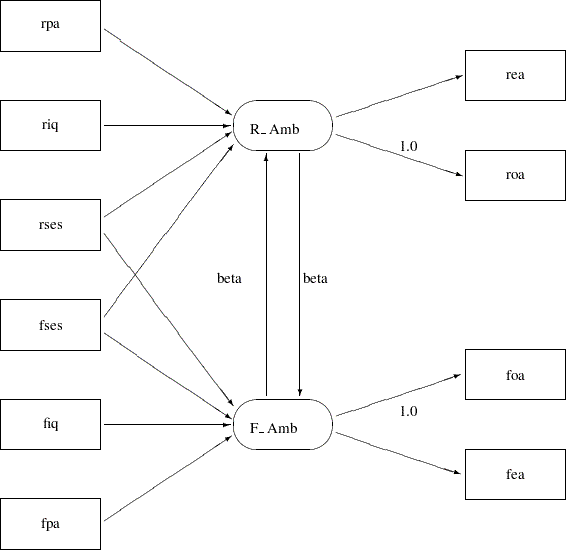
In Figure 17.40, the double-headed path that connected R_Amb and F_Amb no longer exists. Also, the single-headed paths between R_Amb and F_Amb are both labeled with beta, indicating the required constrained effects in the model. The path diagram in Figure 17.40 is transcribed into the PATH model in the following statements:
proc calis data=aspire nobs=329;
   path
      /* structural model of influences */
      rpa    ---> R_Amb         ,
      riq    ---> R_Amb         ,
      rses   ---> R_Amb         ,
      fses   ---> R_Amb         ,
      rses   ---> F_Amb         ,
      fses   ---> F_Amb         ,
      fiq    ---> F_Amb         ,
      fpa    ---> F_Amb         ,
      F_Amb  ---> R_Amb   = beta,
      R_Amb  ---> F_Amb   = beta,

      /* measurement model for aspiration */
      R_Amb  ---> rea         ,
      R_Amb  ---> roa     = 1.,
      F_Amb  ---> foa     = 1.,
      F_Amb  ---> fea     ;
run;
The only differences between the current specification and the preceding specification for Analysis 1 are the labeling of two paths with the same parameter beta and the deletion of PCOV statement where the covariance of R_Amb and F_Amb was specified in Analysis 1. The fit summary of the current model is displayed in Figure 17.41, and the estimation results are displayed in Figure 17.42.
The model fit chi-square value is 26.8987 (=17, =0.0596). The standardized RMSR and the RMSEA are both less than 0.05, while the adjusted GFI and comparative fit index are both bigger than 0.9. All these indicate a good model fit, but how does this model (Analysis 2) compare with that in Analysis 1?
The difference between the chi-square values for Analyses 1 and 2 is  with two degrees of freedom, which is far from significant. This indicates that the restricted model (Analysis 2) fits as well as the unrestricted model (Analysis 1). The AIC is 102.8987, and the SBC is 247.149. Both of these values are smaller than that of Analysis 1 (106.697 for AIC and 258.540 for SBC), and hence they indicate that the current model is a better one.
| PATH List | ||||||
|---|---|---|---|---|---|---|
| Path | Parameter | Estimate | Standard Error |
t Value | ||
| rpa | ---> | R_Amb | _Parm01 | 0.16367 | 0.03872 | 4.22740 |
| riq | ---> | R_Amb | _Parm02 | 0.25395 | 0.04186 | 6.06726 |
| rses | ---> | R_Amb | _Parm03 | 0.22115 | 0.04187 | 5.28218 |
| fses | ---> | R_Amb | _Parm04 | 0.07728 | 0.04149 | 1.86264 |
| rses | ---> | F_Amb | _Parm05 | 0.06840 | 0.03868 | 1.76809 |
| fses | ---> | F_Amb | _Parm06 | 0.21839 | 0.03948 | 5.53198 |
| fiq | ---> | F_Amb | _Parm07 | 0.33063 | 0.04116 | 8.03314 |
| fpa | ---> | F_Amb | _Parm08 | 0.15204 | 0.03636 | 4.18169 |
| F_Amb | ---> | R_Amb | beta | 0.18007 | 0.03912 | 4.60305 |
| R_Amb | ---> | F_Amb | beta | 0.18007 | 0.03912 | 4.60305 |
| R_Amb | ---> | rea | _Parm09 | 1.06097 | 0.08921 | 11.89233 |
| R_Amb | ---> | roa | 1.00000 | |||
| F_Amb | ---> | foa | 1.00000 | |||
| F_Amb | ---> | fea | _Parm10 | 1.07359 | 0.08063 | 13.31498 |
| Variance Parameters | |||||
|---|---|---|---|---|---|
| Variance Type |
Variable | Parameter | Estimate | Standard Error |
t Value |
| Exogenous | riq | _Add01 | 1.00000 | 0.07809 | 12.80625 |
| rpa | _Add02 | 1.00000 | 0.07809 | 12.80625 | |
| rses | _Add03 | 1.00000 | 0.07809 | 12.80625 | |
| fiq | _Add04 | 1.00000 | 0.07809 | 12.80625 | |
| fpa | _Add05 | 1.00000 | 0.07809 | 12.80625 | |
| fses | _Add06 | 1.00000 | 0.07809 | 12.80625 | |
| Error | roa | _Add07 | 0.41205 | 0.05103 | 8.07403 |
| rea | _Add08 | 0.33764 | 0.05178 | 6.52039 | |
| foa | _Add09 | 0.40381 | 0.04608 | 8.76427 | |
| fea | _Add10 | 0.31337 | 0.04574 | 6.85166 | |
| R_Amb | _Add11 | 0.28113 | 0.04640 | 6.05867 | |
| F_Amb | _Add12 | 0.22924 | 0.03889 | 5.89393 | |
| Covariances Among Exogenous Variables | |||||
|---|---|---|---|---|---|
| Var1 | Var2 | Parameter | Estimate | Standard Error |
t Value |
| rpa | riq | _Add13 | 0.18390 | 0.05614 | 3.27564 |
| rses | riq | _Add14 | 0.22200 | 0.05656 | 3.92503 |
| rses | rpa | _Add15 | 0.04890 | 0.05528 | 0.88456 |
| fiq | riq | _Add16 | 0.33550 | 0.05824 | 5.76060 |
| fiq | rpa | _Add17 | 0.07820 | 0.05538 | 1.41195 |
| fiq | rses | _Add18 | 0.23020 | 0.05666 | 4.06284 |
| fpa | riq | _Add19 | 0.10210 | 0.05550 | 1.83955 |
| fpa | rpa | _Add20 | 0.11470 | 0.05558 | 2.06377 |
| fpa | rses | _Add21 | 0.09310 | 0.05545 | 1.67885 |
| fpa | fiq | _Add22 | 0.20870 | 0.05641 | 3.70000 |
| fses | riq | _Add23 | 0.18610 | 0.05616 | 3.31352 |
| fses | rpa | _Add24 | 0.01860 | 0.05523 | 0.33680 |
| fses | rses | _Add25 | 0.27070 | 0.05720 | 4.73226 |
| fses | fiq | _Add26 | 0.29500 | 0.05757 | 5.12435 |
| fses | fpa | _Add27 | -0.04380 | 0.05527 | -0.79249 |
Like Analysis 1, the same two paths in the current analysis are not significant. That is, fses does not seem to be a good indicator of a respondent’s ambition R_Amb, and rses does not seem to be a good indicator of a friend’s ambition F_Amb. The values are 1.862 and 1.768, respectively.
Career Aspiration: Analysis 3
Loehlin (1987) points out that the models considered are unrealistic in at least two respects. First, the variables of parental aspiration, intelligence, and socioeconomic status are assumed to be measured without error. Loehlin adds uncorrelated measurement errors to the model and assumes, for illustrative purposes, that the reliabilities of these variables are known to be 0.7, 0.8, and 0.9, respectively. In practice, these reliabilities would need to be obtained from a separate study of the same or a very similar population. If these constraints are omitted, the model is not identified. However, constraining parameters to a constant in an analysis of a correlation matrix might make the chi-square goodness-of-fit test inaccurate, so there is more reason to be skeptical of the -values. Second, the error terms for the respondent’s aspiration are assumed to be uncorrelated with the corresponding terms for his friend. Loehlin introduces a correlation between the two educational aspiration error terms and between the two occupational aspiration error terms. These additions produce the path diagram for Loehlin’s model shown in Figure 17.43.
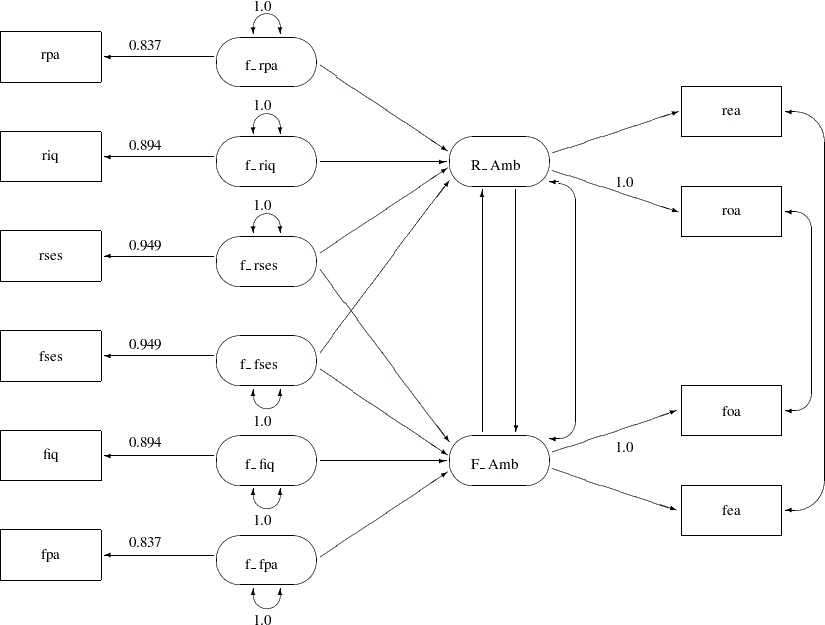
In Figure 17.43, the observed variables rpa, riq, rses, fses, fiq, and fpa are all measured with measurement errors. Their true scores counterparts f_rpa, f_riq, f_rses, f_fses, f_fiq, and f_fpa are latent variables in the model. Path coefficients from these latent variables to the observed variables are fixed coefficients, indicating the square roots of the theoretical reliabilities in the model. These latent variables, rather than the observed counterparts, serve as predictors of the ambition factors R_Amb and F_Amb in the current model (Analysis 3). The error terms for these two latent factors are correlated, as indicated by a double-headed path (arrow) that connects the two factors. Correlated errors for the occupational aspiration variables (roa and foa) and the educational aspiration variables (rea and fea) are also shown in Figure 17.43. Again, these correlated errors are represented by two double-headed paths (arrows) in the path diagram.
You use the following statements to specify the path model for Analysis 3:
proc calis data=aspire nobs=329;
   path
      /* measurement model for intelligence and environment */
      rpa     <---  f_rpa    = 0.837,
      riq     <---  f_riq    = 0.894,
      rses    <---  f_rses   = 0.949,
      fses    <---  f_fses   = 0.949,
      fiq     <---  f_fiq    = 0.894,
      fpa     <---  f_fpa    = 0.837,

      /* structural model of influences */
      f_rpa   --->  R_Amb,
      f_riq   --->  R_Amb,
      f_rses  --->  R_Amb,
      f_fses  --->  R_Amb,
      f_rses  --->  F_Amb,
      f_fses  --->  F_Amb,
      f_fiq   --->  F_Amb,
      f_fpa   --->  F_Amb,
      F_Amb   --->  R_Amb,
      R_Amb   --->  F_Amb,

      /* measurement model for aspiration */
      R_Amb   --->  rea        ,
      R_Amb   --->  roa    = 1.,
      F_Amb   --->  foa    = 1.,
      F_Amb   --->  fea    ;
   pvar
      f_rpa f_riq f_rses f_fses f_fiq f_fpa = 6 * 1.0;
   pcov
      R_Amb F_Amb  ,
      rea  fea     ,
      roa  foa     ;
run;
In this specification, the measurement model for the six intelligence and environment variables are added. They are the first six paths in the PATH statement. Fixed constants are set for these path coefficients so as to make the measurement model identified and to set the required reliabilities of these measurement indicators. The structural model of influences and the measurement model for aspiration are the same as specified in Analysis 1. (See the section Career Aspiration: Analysis 1.) All the correlated errors are specified in the PCOV statement.
The fit summary of the current model is displayed in Figure 17.44.
Since the -value for the chi-square test is 0.5266, this model clearly cannot be rejected. Both the standardized RMSR and the RMSEA are very small, and both the adjusted GFI and the comparative fit index are high. All these point to an excellent model fit. However, Schwarz’s Bayesian criterion for this model (SBC = 255.4476) is somewhat larger than for Jöreskog and Sörbom (1988) Analysis 2 in Figure 17.41 (SBC = 247.1489), suggesting that a more parsimonious model would be desirable.
The estimation results are displayed in Figure 17.45.
| PATH List | ||||||
|---|---|---|---|---|---|---|
| Path | Parameter | Estimate | Standard Error |
t Value | ||
| rpa | <--- | f_rpa | 0.83700 | |||
| riq | <--- | f_riq | 0.89400 | |||
| rses | <--- | f_rses | 0.94900 | |||
| fses | <--- | f_fses | 0.94900 | |||
| fiq | <--- | f_fiq | 0.89400 | |||
| fpa | <--- | f_fpa | 0.83700 | |||
| f_rpa | ---> | R_Amb | _Parm01 | 0.18370 | 0.05044 | 3.64201 |
| f_riq | ---> | R_Amb | _Parm02 | 0.28004 | 0.06139 | 4.56183 |
| f_rses | ---> | R_Amb | _Parm03 | 0.22616 | 0.05223 | 4.33004 |
| f_fses | ---> | R_Amb | _Parm04 | 0.08698 | 0.05476 | 1.58836 |
| f_rses | ---> | F_Amb | _Parm05 | 0.06327 | 0.05219 | 1.21240 |
| f_fses | ---> | F_Amb | _Parm06 | 0.21539 | 0.05121 | 4.20600 |
| f_fiq | ---> | F_Amb | _Parm07 | 0.35386 | 0.06741 | 5.24971 |
| f_fpa | ---> | F_Amb | _Parm08 | 0.16877 | 0.04934 | 3.42051 |
| F_Amb | ---> | R_Amb | _Parm09 | 0.11897 | 0.11396 | 1.04397 |
| R_Amb | ---> | F_Amb | _Parm10 | 0.13022 | 0.12067 | 1.07921 |
| R_Amb | ---> | rea | _Parm11 | 1.08398 | 0.09417 | 11.51054 |
| R_Amb | ---> | roa | 1.00000 | |||
| F_Amb | ---> | foa | 1.00000 | |||
| F_Amb | ---> | fea | _Parm12 | 1.11631 | 0.08627 | 12.93937 |
| Variance Parameters | |||||
|---|---|---|---|---|---|
| Variance Type |
Variable | Parameter | Estimate | Standard Error |
t Value |
| Exogenous | f_rpa | 1.00000 | |||
| f_riq | 1.00000 | ||||
| f_rses | 1.00000 | ||||
| f_fses | 1.00000 | ||||
| f_fiq | 1.00000 | ||||
| f_fpa | 1.00000 | ||||
| Error | riq | _Add01 | 0.20874 | 0.07832 | 2.66519 |
| rpa | _Add02 | 0.29584 | 0.07774 | 3.80573 | |
| rses | _Add03 | 0.09887 | 0.07803 | 1.26715 | |
| roa | _Add04 | 0.42307 | 0.05243 | 8.06948 | |
| rea | _Add05 | 0.32707 | 0.05452 | 5.99883 | |
| fiq | _Add06 | 0.19988 | 0.07674 | 2.60475 | |
| fpa | _Add07 | 0.29987 | 0.07807 | 3.84089 | |
| fses | _Add08 | 0.10324 | 0.07824 | 1.31950 | |
| foa | _Add09 | 0.42240 | 0.04730 | 8.93103 | |
| fea | _Add10 | 0.28715 | 0.04804 | 5.97748 | |
| R_Amb | _Add11 | 0.25418 | 0.04469 | 5.68738 | |
| F_Amb | _Add12 | 0.19698 | 0.03814 | 5.16533 | |
| Covariances Among Exogenous Variables | |||||
|---|---|---|---|---|---|
| Var1 | Var2 | Parameter | Estimate | Standard Error |
t Value |
| f_riq | f_rpa | _Add13 | 0.24677 | 0.07519 | 3.28204 |
| f_rses | f_rpa | _Add14 | 0.06184 | 0.06945 | 0.89034 |
| f_rses | f_riq | _Add15 | 0.26351 | 0.06687 | 3.94075 |
| f_fses | f_rpa | _Add16 | 0.02383 | 0.06952 | 0.34272 |
| f_fses | f_riq | _Add17 | 0.22135 | 0.06648 | 3.32976 |
| f_fses | f_rses | _Add18 | 0.30156 | 0.06359 | 4.74205 |
| f_fiq | f_rpa | _Add19 | 0.10853 | 0.07362 | 1.47419 |
| f_fiq | f_riq | _Add20 | 0.42476 | 0.07219 | 5.88373 |
| f_fiq | f_rses | _Add21 | 0.27250 | 0.06660 | 4.09143 |
| f_fiq | f_fses | _Add22 | 0.34922 | 0.06771 | 5.15755 |
| f_fpa | f_rpa | _Add23 | 0.15789 | 0.07873 | 2.00553 |
| f_fpa | f_riq | _Add24 | 0.13085 | 0.07418 | 1.76393 |
| f_fpa | f_rses | _Add25 | 0.11517 | 0.06978 | 1.65053 |
| f_fpa | f_fses | _Add26 | -0.05623 | 0.06971 | -0.80655 |
| f_fpa | f_fiq | _Add27 | 0.27867 | 0.07530 | 3.70083 |
Like Analyses 1 and 2, two paths that concern the validity of the indicators in the current analysis do not show significance. That is, f_fses does not seem to be a good indicator of a respondent’s ambition R_Amb, and f_rses does not seem to be a good indicator of a friend’s ambition F_Amb. The values are 1.588 and 1.212, respectively. In addition, in the current model (Analysis 3), the structural relationships between the ambition factors do not show significance. The value for the path from the friend’s ambition factor F_Amb on the respondent’s ambition factor R_Amb is only 1.044, while the value for the path from the respondent’s ambition factor R_Amb on the friend’s ambition factor F_Amb is only 1.079. These cast doubts on the validity of the structural model and perhaps even the entire model.
Copyright © SAS Institute, Inc. All Rights Reserved.