Residual Panels

There are three types of residual panels in the GLIMMIX procedure. Their makeup of four component plots is the same; the difference lies in the type of residual from which the panel is computed. Raw residuals are displayed with the PLOTS=RESIDUALPANEL option. Studentized residuals are displayed with the PLOTS=STUDENTPANEL option, and Pearson residuals with the PLOTS==PEARSONPANEL option. By default, conditional residuals are used in the construction of the panels if the model contains G-side random effects. For example, consider the following statements:

proc glimmix plots=residualpanel;
   class A;
   model y = x1 x2 / dist=Poisson;
   random int / sub=A;
run;

The parameters are estimated by a pseudo-likelihood method, and at the final stage pseudo-data are related to a linear mixed model with random intercepts. The residual panel is constructed from

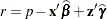where is the pseudo-data.

The following hypothetical data set contains yields of an industrial process. Material was available from five randomly selected vendors to produce a chemical reaction whose yield depends on two factors (pressure and temperature at 3 and 2 levels, respectively).

 data Yields;
   input Vendor Pressure Temp Yield @@;
   datalines;
 1  1  1  10.20    1  1  2   9.48    1  2  1   9.74  
 1  2  2   8.92    1  3  1  11.79    1  3  2   8.85  
 2  1  1  10.43    2  1  2  10.59    2  2  1  10.29 
 2  2  2  10.15    2  3  1  11.12    2  3  2   9.30  
 3  1  1   6.46    3  1  2   7.34    3  2  1   9.44 
 3  2  2   8.11    3  3  1   9.38    3  3  2   8.37 
 4  1  1   7.36    4  1  2   9.92    4  2  1  10.99 
 4  2  2  10.34    4  3  1  10.24    4  3  2   9.96 
 5  1  1  11.72    5  1  2  10.60    5  2  1  11.28 
 5  2  2   9.03    5  3  1  14.09    5  3  2   8.92 
;

We consider here a linear mixed model with a two-way factorial fixed-effects structure for pressure and temperature effects and independent, homoscedastic random effects for the vendors. The following statements fit this model and request panels of marginal and conditional residuals:

ods graphics on;

proc glimmix data=Yields 
      plots=residualpanel(conditional marginal);
   class Vendor Pressure Temp;
   model Yield = Pressure Temp Pressure*Temp;
   random vendor;
run;

ods graphics off;

The suboptions of the RESIDUALPANEL request produce two panels. The panel of conditional residuals is constructed from (Figure 38.19). The panel of marginal residuals is constructed from (Figure 38.20). Note that these residuals are deviations from the observed data, because the model is a normal linear mixed model, and hence it does not involve pseudo-data. Whenever the random-effects solutions are involved in constructing residuals, the title of the residual graphics identifies them as conditional residuals (Figure 38.19).

Figure 38.19 Conditional Residuals

Figure 38.20 Marginal Residuals

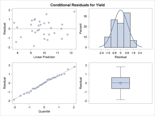
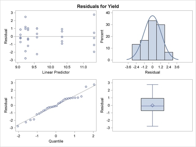
The predictor takes on only six values for the marginal residuals, corresponding to the combinations of three temperature and two pressure levels. The assumption of a zero mean for the vendor random effect seems justified; the marginal residuals in the upper-left plot of Figure 38.20 do not exhibit any trend. The conditional residuals in Figure 38.19 are smaller and somewhat closer to normality compared to the marginal residuals.

Box Plots

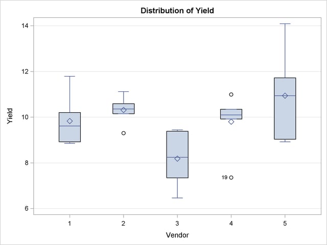
You can produce box plots of observed data, pseudo-data, and various residuals for effects in your model that consist of classification variables. Because you might not want to produce box plots for all such effects, you can request subsets with the suboptions of the BOXPLOT option in the PLOTS option. The BOXPLOT request in the following PROC GLIMMIX statement produces box plots for the random effects—in this case, the vendor effect. By default, PROC GLIMMIX constructs box plots from conditional residuals. The MARGINAL, CONDITIONAL, and OBSERVED suboptions instruct the procedure to construct three box plots for each random effect: box plots of the observed data (Figure 38.21), the marginal residuals (Figure 38.22), and the conditional residuals (Figure 38.23).

ods graphics on;

proc glimmix data=Yields 
       plots=boxplot(random marginal conditional observed);
   class Vendor Pressure Temp;
   model Yield = Pressure Temp Pressure*Temp;
   random vendor;
run;

ods graphics off;

The observed vendor means in Figure 38.21 are different; in particular, vendors 3 and 5 appear to differ from the other vendors and from each other. There is also heterogeneity of variance in the five groups. The marginal residuals in Figure 38.22 continue to show the differences in means by vendor, because vendor enters the model as a random effect. The marginal means are adjusted for vendor effects only in the sense that the vendor variance component affects the marginal variance that is involved in the generalized least squares solution for the pressure and temperature effects.

Figure 38.21 Box Plots of Observed Values

Figure 38.22 Box Plots of Marginal Residuals

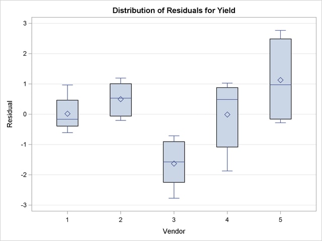
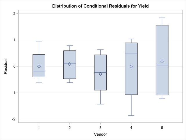
The conditional residuals account for the vendor effects through the empirical BLUPs. The means and medians have stabilized near zero, but some heterogeneity in these residuals remains (Figure 38.23).

Figure 38.23 Box Plots of Conditional Residuals