| The GENMOD Procedure |
Example 37.8 Model Assessment of Multiple Regression Using Aggregates of Residuals
This example illustrates the use of cumulative residuals to assess the adequacy of a normal linear regression model. Neter et al. (1996, Section 8.2) describe a study of 54 patients undergoing a certain kind of liver operation in a surgical unit. The data consist of the survival time and certain covariates. After a model selection procedure, they arrived at the following model:
 |
where  is the logarithm (base 10) of the survival time;
  ,
,  ,
,  are blood-clotting score, prognostic index, and enzyme function, respectively; and
  is a normal error term. A listing of the SAS data set containing the data is shown in Output 37.8.1. The variables Y, X1, X2, and X3 correspond to , , , and , and LogX1 is log(). The PROC GENMOD fit of the model is shown in Output 37.8.2. The analysis first focuses on the adequacy of the functional form of , blood-clotting score.
| Obs | Y | X1 | X2 | X3 | LogX1 |
|---|---|---|---|---|---|
| 1 | 2.3010 | 6.7 | 62 | 81 | 0.82607 |
| 2 | 2.0043 | 5.1 | 59 | 66 | 0.70757 |
| 3 | 2.3096 | 7.4 | 57 | 83 | 0.86923 |
| 4 | 2.0043 | 6.5 | 73 | 41 | 0.81291 |
| 5 | 2.7067 | 7.8 | 65 | 115 | 0.89209 |
| 6 | 1.9031 | 5.8 | 38 | 72 | 0.76343 |
| 7 | 1.9031 | 5.7 | 46 | 63 | 0.75587 |
| 8 | 2.1038 | 3.7 | 68 | 81 | 0.56820 |
| 9 | 2.3054 | 6.0 | 67 | 93 | 0.77815 |
| 10 | 2.3075 | 3.7 | 76 | 94 | 0.56820 |
| 11 | 2.5172 | 6.3 | 84 | 83 | 0.79934 |
| 12 | 1.8129 | 6.7 | 51 | 43 | 0.82607 |
| 13 | 2.9191 | 5.8 | 96 | 114 | 0.76343 |
| 14 | 2.5185 | 5.8 | 83 | 88 | 0.76343 |
| 15 | 2.2253 | 7.7 | 62 | 67 | 0.88649 |
| 16 | 2.3365 | 7.4 | 74 | 68 | 0.86923 |
| 17 | 1.9395 | 6.0 | 85 | 28 | 0.77815 |
| 18 | 1.5315 | 3.7 | 51 | 41 | 0.56820 |
| 19 | 2.3324 | 7.3 | 68 | 74 | 0.86332 |
| 20 | 2.2355 | 5.6 | 57 | 87 | 0.74819 |
| 21 | 2.0374 | 5.2 | 52 | 76 | 0.71600 |
| 22 | 2.1335 | 3.4 | 83 | 53 | 0.53148 |
| 23 | 1.8451 | 6.7 | 26 | 68 | 0.82607 |
| 24 | 2.3424 | 5.8 | 67 | 86 | 0.76343 |
| 25 | 2.4409 | 6.3 | 59 | 100 | 0.79934 |
| 26 | 2.1584 | 5.8 | 61 | 73 | 0.76343 |
| 27 | 2.2577 | 5.2 | 52 | 86 | 0.71600 |
| 28 | 2.7589 | 11.2 | 76 | 90 | 1.04922 |
| 29 | 1.8573 | 5.2 | 54 | 56 | 0.71600 |
| 30 | 2.2504 | 5.8 | 76 | 59 | 0.76343 |
| 31 | 1.8513 | 3.2 | 64 | 65 | 0.50515 |
| 32 | 1.7634 | 8.7 | 45 | 23 | 0.93952 |
| 33 | 2.0645 | 5.0 | 59 | 73 | 0.69897 |
| 34 | 2.4698 | 5.8 | 72 | 93 | 0.76343 |
| 35 | 2.0607 | 5.4 | 58 | 70 | 0.73239 |
| 36 | 2.2648 | 5.3 | 51 | 99 | 0.72428 |
| 37 | 2.0719 | 2.6 | 74 | 86 | 0.41497 |
| 38 | 2.0792 | 4.3 | 8 | 119 | 0.63347 |
| 39 | 2.1790 | 4.8 | 61 | 76 | 0.68124 |
| 40 | 2.1703 | 5.4 | 52 | 88 | 0.73239 |
| 41 | 1.9777 | 5.2 | 49 | 72 | 0.71600 |
| 42 | 1.8751 | 3.6 | 28 | 99 | 0.55630 |
| 43 | 2.6840 | 8.8 | 86 | 88 | 0.94448 |
| 44 | 2.1847 | 6.5 | 56 | 77 | 0.81291 |
| 45 | 2.2810 | 3.4 | 77 | 93 | 0.53148 |
| 46 | 2.0899 | 6.5 | 40 | 84 | 0.81291 |
| 47 | 2.4928 | 4.5 | 73 | 106 | 0.65321 |
| 48 | 2.5999 | 4.8 | 86 | 101 | 0.68124 |
| 49 | 2.1987 | 5.1 | 67 | 77 | 0.70757 |
| 50 | 2.4914 | 3.9 | 82 | 103 | 0.59106 |
| 51 | 2.0934 | 6.6 | 77 | 46 | 0.81954 |
| 52 | 2.0969 | 6.4 | 85 | 40 | 0.80618 |
| 53 | 2.2967 | 6.4 | 59 | 85 | 0.80618 |
| 54 | 2.4955 | 8.8 | 78 | 72 | 0.94448 |
In order to assess the adequacy of the fitted multiple regression model, the ASSESS statement in the following SAS statements is used to create the plots of cumulative residuals against X1 shown in Output 37.8.3 and Output 37.8.4 and the summary table in Output 37.8.5:
ods graphics on;
proc genmod data=Surg;
   model Y = X1 X2 X3 / scale=Pearson;
   assess var=(X1) / resample=10000
                     seed=603708000
                     crpanel ;
run;
| Analysis Of Maximum Likelihood Parameter Estimates | |||||||
|---|---|---|---|---|---|---|---|
| Parameter | DF | Estimate | Standard Error | Wald 95% Confidence Limits | Wald Chi-Square | Pr > ChiSq | |
| Intercept | 1 | 0.4836 | 0.0426 | 0.4001 | 0.5672 | 128.71 | <.0001 |
| X1 | 1 | 0.0692 | 0.0041 | 0.0612 | 0.0772 | 288.17 | <.0001 |
| X2 | 1 | 0.0093 | 0.0004 | 0.0085 | 0.0100 | 590.45 | <.0001 |
| X3 | 1 | 0.0095 | 0.0003 | 0.0089 | 0.0101 | 966.07 | <.0001 |
| Scale | 0 | 0.0469 | 0.0000 | 0.0469 | 0.0469 | ||
| Note: | The scale parameter was estimated by the square root of Pearson's Chi-Square/DOF. |
See Lin, Wei, and Ying (2002) for details about model assessment that uses cumulative residual plots. The RESAMPLE= keyword specifies that a  -value be computed based on a sample of 10,000 simulated residual paths. A random number seed is specified by the SEED= keyword for reproducibility. If you do not specify the seed, one is derived from the time of day. The keyword CRPANEL specifies that the panel of four cumulative residual plots shown in Output 37.8.4 be created, each with two simulated paths. The single residual plot with 20 simulated paths in Output 37.8.3 is created by default.
These graphical displays are requested by specifying the ODS GRAPHICS statement and the ASSESS statement. For general information about ODS Graphics, see Chapter 21, Statistical Graphics Using ODS. For specific information about the graphics available in the GENMOD procedure, see the section ODS Graphics.
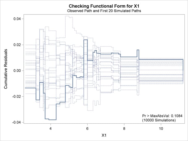
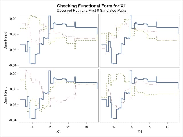
The -value of 0.1084 reported on Output 37.8.3 and Output 37.8.5 suggests that a more adequate model might be possible. The observed cumulative residuals in Output 37.8.3 and Output 37.8.4, represented by the heavy lines, seem atypical of the simulated curves, represented by the light lines, reinforcing the conclusion that a more appropriate functional form for X1 is possible.
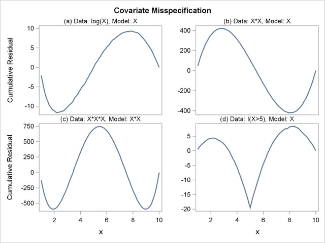
The cumulative residual plots in Output 37.8.6 provide guidance in determining a more appropriate functional form. The four curves were created from simple forms of model misspecification by using simulated data. The mean models of the data and the fitted model are shown in Table 37.15.
Plot |
Data E( |
Fitted Model E( |
|---|---|---|
(a) |
log( |
|
(b) |
|
|
(c) |
|
|
(d) |
|
|
 )
) 


The observed cumulative residual pattern in Output 37.8.3 and Output 37.8.4 most resembles the behavior of the curve in plot (a) of Output 37.8.6, indicating that log() might be a more appropriate term in the model than .
The following SAS statements fit a model with LogX1 in place of X1 and request a model assessment:
proc genmod data=Surg;
   model Y = LogX1 X2 X3 / scale=Pearson;
   assess var=(LogX1) / resample=10000
                        seed=603708000;
run;
ods graphics off;
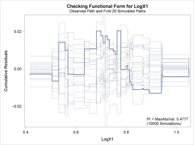
The revised model fit is shown in Output 37.8.7, the -value from the simulation is 0.4777, and the cumulative residuals plotted in Output 37.8.8 show no systematic trend. The log transformation for X1 is more appropriate. Under the revised model, the -values for testing the functional forms of X2 and X3 are 0.20 and 0.63, respectively; and the -value for testing the linearity of the model is 0.65. Thus, the revised model seems reasonable.
| Analysis Of Maximum Likelihood Parameter Estimates | |||||||
|---|---|---|---|---|---|---|---|
| Parameter | DF | Estimate | Standard Error | Wald 95% Confidence Limits | Wald Chi-Square | Pr > ChiSq | |
| Intercept | 1 | 0.1844 | 0.0504 | 0.0857 | 0.2832 | 13.41 | 0.0003 |
| LogX1 | 1 | 0.9121 | 0.0491 | 0.8158 | 1.0083 | 345.05 | <.0001 |
| X2 | 1 | 0.0095 | 0.0004 | 0.0088 | 0.0102 | 728.62 | <.0001 |
| X3 | 1 | 0.0096 | 0.0003 | 0.0090 | 0.0101 | 1139.73 | <.0001 |
| Scale | 0 | 0.0434 | 0.0000 | 0.0434 | 0.0434 | ||
| Note: | The scale parameter was estimated by the square root of Pearson's Chi-Square/DOF. |
Copyright © SAS Institute, Inc. All Rights Reserved.