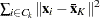
Average Linkage

The following method is obtained by specifying METHOD=AVERAGE. The distance between two clusters is defined by

If , then

The combinatorial formula is

In average linkage the distance between two clusters is the average distance between pairs of observations, one in each cluster. Average linkage tends to join clusters with small variances, and it is slightly biased toward producing clusters with the same variance.

Average linkage was originated by Sokal and Michener (1958).

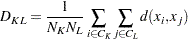
Centroid Method

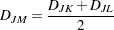
The following method is obtained by specifying METHOD=CENTROID. The distance between two clusters is defined by

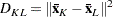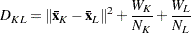
If , then the combinatorial formula is

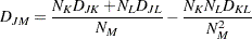In the centroid method, the distance between two clusters is defined as the (squared) Euclidean distance between their centroids or means. The centroid method is more robust to outliers than most other hierarchical methods but in other respects might not perform as well as Ward’s method or average linkage (Milligan; 1980).

The centroid method was originated by Sokal and Michener (1958).

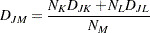
Complete Linkage

The following method is obtained by specifying METHOD=COMPLETE. The distance between two clusters is defined by

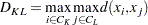The combinatorial formula is

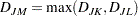In complete linkage, the distance between two clusters is the maximum distance between an observation in one cluster and an observation in the other cluster. Complete linkage is strongly biased toward producing clusters with roughly equal diameters, and it can be severely distorted by moderate outliers (Milligan; 1980).

Complete linkage was originated by Sorensen (1948).

Density Linkage

The phrase density linkage is used here to refer to a class of clustering methods that use nonparametric probability density estimates (for example, Hartigan; 1975, pp. 205–212; Wong 1982; Wong and Lane 1983). Density linkage consists of two steps:

1. A new dissimilarity measure, , based on density estimates and adjacencies is computed. If and are adjacent (the definition of adjacency depends on the method of density estimation), then is the reciprocal of an estimate of the density midway between and ; otherwise, is infinite.

2. A single linkage cluster analysis is performed using .

The CLUSTER procedure supports three types of density linkage: the th-nearest-neighbor method, the uniform-kernel method, and Wong’s hybrid method. These are obtained by using METHOD=DENSITY and the K=, R=, and HYBRID options, respectively.

kth-Nearest-Neighbor Method

The th-nearest-neighbor method (Wong and Lane; 1983) uses th-nearest-neighbor density estimates. Let be the distance from point to the th-nearest observation, where is the value specified for the K= option. Consider a closed sphere centered at with radius . The estimated density at , , is the proportion of observations within the sphere divided by the volume of the sphere. The new dissimilarity measure is computed as

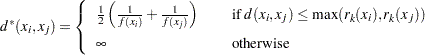Wong and Lane (1983) show that th-nearest-neighbor density linkage is strongly set consistent for high-density (density-contour) clusters if is chosen such that and as . Wong and Schaack (1982) discuss methods for estimating the number of population clusters by using th-nearest-neighbor clustering.

Uniform-Kernel Method

The uniform-kernel method uses uniform-kernel density estimates. Let be the value specified for the R= option. Consider a closed sphere centered at point with radius . The estimated density at , , is the proportion of observations within the sphere divided by the volume of the sphere. The new dissimilarity measure is computed as

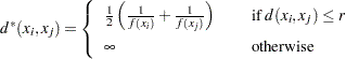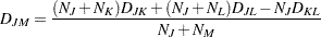
Wong’s Hybrid Method

The Wong (1982) hybrid clustering method uses density estimates based on a preliminary cluster analysis by the -means method. The preliminary clustering can be done by the FASTCLUS procedure, by using the MEAN= option to create a data set containing cluster means, frequencies, and root mean squared standard deviations. This data set is used as input to the CLUSTER procedure, and the HYBRID option is specified with METHOD=DENSITY to request the hybrid analysis. The hybrid method is appropriate for very large data sets but should not be used with small data sets—say, than those with fewer than 100 observations in the original data. The term preliminary cluster refers to an observation in the DATA= data set.

For preliminary cluster , and are obtained from the input data set, as are the cluster means or the distances between the cluster means. Preliminary clusters and are considered adjacent if the midpoint between and is closer to either or than to any other preliminary cluster mean or, equivalently, if for all other preliminary clusters , or . The new dissimilarity measure is computed as

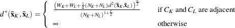Using the K= and R= Options

The values of the K= and R= options are called smoothing parameters. Small values of K= or R= produce jagged density estimates and, as a consequence, many modes. Large values of K= or R= produce smoother density estimates and fewer modes. In the hybrid method, the smoothing parameter is the number of clusters in the preliminary cluster analysis. The number of modes in the final analysis tends to increase as the number of clusters in the preliminary analysis increases. Wong (1982) suggests using preliminary clusters, where is the number of observations in the original data set. There is no rule of thumb for selecting K= values. For all types of density linkage, you should repeat the analysis with several different values of the smoothing parameter (Wong and Schaack; 1982).

There is no simple answer to the question of which smoothing parameter to use (Silverman; 1986, pp. 43–61, 84–88, and 98–99). It is usually necessary to try several different smoothing parameters. A reasonable first guess for the R= option in many coordinate data sets is given by

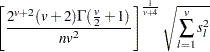where is the standard deviation of the th variable. The estimate for R= can be computed in a DATA step by using the GAMMA function for . This formula is derived under the assumption that the data are sampled from a multivariate normal distribution and tends, therefore, to be too large (oversmooth) if the true distribution is multimodal. Robust estimates of the standard deviations can be preferable if there are outliers. If the data are distances, the factor can be replaced by an average (mean, trimmed mean, median, root mean square, and so on) distance divided by . To prevent outliers from appearing as separate clusters, you can also specify K=2, or more generally K=, , which in most cases forces clusters to have at least members.

If the variables all have unit variance (for example, if the STANDARD option is used), Table 29.2 can be used to obtain an initial guess for the R= option.

Since infinite values occur in density linkage, the final number of clusters can exceed one when there are wide gaps between the clusters or when the smoothing parameter results in little smoothing.

Density linkage applies no constraints to the shapes of the clusters and, unlike most other hierarchical clustering methods, is capable of recovering clusters with elongated or irregular shapes. Since density linkage uses less prior knowledge about the shape of the clusters than do methods restricted to compact clusters, density linkage is less effective at recovering compact clusters from small samples than are methods that always recover compact clusters, regardless of the data.

Table 29.2 Reasonable First Guess for the R= Option for Standardized Data

Number of	Number of Variables
Observations	1	2	3	4	5	6	7	8	9	10
20	1.01	1.36	1.77	2.23	2.73	3.25	3.81	4.38	4.98	5.60
35	0.91	1.24	1.64	2.08	2.56	3.08	3.62	4.18	4.77	5.38
50	0.84	1.17	1.56	1.99	2.46	2.97	3.50	4.06	4.64	5.24
75	0.78	1.09	1.47	1.89	2.35	2.85	3.38	3.93	4.50	5.09
100	0.73	1.04	1.41	1.82	2.28	2.77	3.29	3.83	4.40	4.99
150	0.68	0.97	1.33	1.73	2.18	2.66	3.17	3.71	4.27	4.85
200	0.64	0.93	1.28	1.67	2.11	2.58	3.09	3.62	4.17	4.75
350	0.57	0.85	1.18	1.56	1.98	2.44	2.93	3.45	4.00	4.56
500	0.53	0.80	1.12	1.49	1.91	2.36	2.84	3.35	3.89	4.45
750	0.49	0.74	1.06	1.42	1.82	2.26	2.74	3.24	3.77	4.32
1000	0.46	0.71	1.01	1.37	1.77	2.20	2.67	3.16	3.69	4.23
1500	0.43	0.66	0.96	1.30	1.69	2.11	2.57	3.06	3.57	4.11
2000	0.40	0.63	0.92	1.25	1.63	2.05	2.50	2.99	3.49	4.03

EML

The following method is obtained by specifying METHOD=EML. The distance between two clusters is given by

The EML method joins clusters to maximize the likelihood at each level of the hierarchy under the following assumptions:

• multivariate normal mixture

• equal spherical covariance matrices

• unequal sampling probabilities

The EML method is similar to Ward’s minimum-variance method but removes the bias toward equal-sized clusters. Practical experience has indicated that EML is somewhat biased toward unequal-sized clusters. You can specify the PENALTY= option to adjust the degree of bias. If you specify PENALTY=, the formula is modified to

The EML method was derived by W. S. Sarle of SAS Institute from the maximum likelihood formula obtained by Symons (1981, p. 37, Equation 8) for disjoint clustering. There are currently no other published references on the EML method.

Flexible-Beta Method

The following method is obtained by specifying METHOD=FLEXIBLE. The combinatorial formula is

where is the value of the BETA= option, or by default.

The flexible-beta method was developed by Lance and Williams (1967); see also Milligan (1987).

McQuitty’s Similarity Analysis

The following method is obtained by specifying METHOD=MCQUITTY. The combinatorial formula is

The method was independently developed by Sokal and Michener (1958) and McQuitty (1966).

Median Method

The following method is obtained by specifying METHOD=MEDIAN. If , then the combinatorial formula is

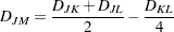The median method was developed by Gower (1967).

Single Linkage

The following method is obtained by specifying METHOD=SINGLE. The distance between two clusters is defined by

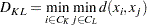The combinatorial formula is

In single linkage, the distance between two clusters is the minimum distance between an observation in one cluster and an observation in the other cluster. Single linkage has many desirable theoretical properties (Jardine and Sibson; 1971; Fisher and Van Ness; 1971; Hartigan; 1981) but has fared poorly in Monte Carlo studies (for example, Milligan 1980). By imposing no constraints on the shape of clusters, single linkage sacrifices performance in the recovery of compact clusters in return for the ability to detect elongated and irregular clusters. You must also recognize that single linkage tends to chop off the tails of distributions before separating the main clusters (Hartigan; 1981). The notorious chaining tendency of single linkage can be alleviated by specifying the TRIM= option (Wishart; 1969, pp. 296–298).

Density linkage and two-stage density linkage retain most of the virtues of single linkage while performing better with compact clusters and possessing better asymptotic properties (Wong and Lane; 1983).

Single linkage was originated by Florek et al. (1951b, 1951a) and later reinvented by McQuitty (1957) and Sneath (1957).

Two-Stage Density Linkage

If you specify METHOD=DENSITY, the modal clusters often merge before all the points in the tails have clustered. The option METHOD=TWOSTAGE is a modification of density linkage that ensures that all points are assigned to modal clusters before the modal clusters are permitted to join. The CLUSTER procedure supports the same three varieties of two-stage density linkage as of ordinary density linkage: th-nearest neighbor, uniform kernel, and hybrid.

In the first stage, disjoint modal clusters are formed. The algorithm is the same as the single linkage algorithm ordinarily used with density linkage, with one exception: two clusters are joined only if at least one of the two clusters has fewer members than the number specified by the MODE= option. At the end of the first stage, each point belongs to one modal cluster.

In the second stage, the modal clusters are hierarchically joined by single linkage. The final number of clusters can exceed one when there are wide gaps between the clusters or when the smoothing parameter is small.

Each stage forms a tree that can be plotted by the TREE procedure. By default, the TREE procedure plots the tree from the first stage. To obtain the tree for the second stage, use the option HEIGHT=MODE in the PROC TREE statement. You can also produce a single tree diagram containing both stages, with the number of clusters as the height axis, by using the option HEIGHT=N in the PROC TREE statement. To produce an output data set from PROC TREE containing the modal clusters, use _HEIGHT_ for the HEIGHT variable (the default) and specify LEVEL=0.

Two-stage density linkage was developed by W. S. Sarle of SAS Institute. There are currently no other published references on two-stage density linkage.

Ward’s Minimum-Variance Method

The following method is obtained by specifying METHOD=WARD. The distance between two clusters is defined by

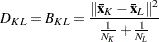If 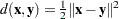, then the combinatorial formula is

In Ward’s minimum-variance method, the distance between two clusters is the ANOVA sum of squares between the two clusters added up over all the variables. At each generation, the within-cluster sum of squares is minimized over all partitions obtainable by merging two clusters from the previous generation. The sums of squares are easier to interpret when they are divided by the total sum of squares to give proportions of variance (squared semipartial correlations).

Ward’s method joins clusters to maximize the likelihood at each level of the hierarchy under the following assumptions:

• multivariate normal mixture

• equal spherical covariance matrices

• equal sampling probabilities

Ward’s method tends to join clusters with a small number of observations, and it is strongly biased toward producing clusters with roughly the same number of observations. It is also very sensitive to outliers (Milligan; 1980).

Ward (1963) describes a class of hierarchical clustering methods including the minimum variance method.