Example 25.13 The Full Information Maximum Likelihood Method
This example shows how you can fully utilize all available information from the data when there is a high proportion of observations with random missing value. You use the full-information maximum likelihood method for model estimation.
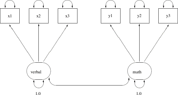
In Example 25.11, 32 students take six tests. These six tests are indicator measures of two ability factors: verbal and math. You conduct a confirmatory factor analysis in Example 25.11 based on a data set without any missing values. The path diagram for the confirmatory factor model is shown the following:
Suppose now due to sickness or unexpected events, some students cannot take part in one of these tests. Now, the data test contains missing values at various locations, as indicated by the following DATA step:
data missing;
   input x1 x2 x3 y1 y2 y3;
   datalines;
 23   .  16  15  14  16
 29  26  23  22  18  19
 14  21   .  15  16  18
 20  18  17  18  21  19
 25  26  22   .  21  26
 26  19  15  16  17  17
  .  17  19   4   6   7
 12  17  18  14  16   .
 25  19  22  22  20  20
  7  12  15  10  11   8
 29  24   .  14  13  16
 28  24  29  19  19  21
 12   9  10  18  19   .
 11   .  12  15  16  16
 20  14  15  24  23  16
 26  25   .  24  23  24
 20  16  19  22  21  20
 14   .  15  17  19  23
 14  20  13  24   .   .
 29  24  24  21  20  18
 26   .  26  28  26  23
 20  23  24  22  23  22
 23  24  20  23  22  18
 14   .  17   .  16  14
 28  34  27  25  21  21
 17  12  10  14  12  16
  .   1  13  14  15  14
 22  19  19  13  11  14
 18  21   .  15  18  19
 12  12  10  13  13  16
 22  14  20  20  18  19
 29  21  22  13  17   .
;
This data set is similar to the scores data set used in Example 25.11, except that some values are replaced at random with missing values. You can still fit the same confirmatory factor-analysis model described in Example 25.11 to this data set by the default maximum likelihood (ML) method, as shown in the following statement:
proc calis data=missing;
   factor
      verbal ---> x1-x3,
      math   ---> y1-y3;
   pvar
      verbal = 1.,
      math   = 1.;
run;
The data set, the number of observations, the model type, and analysis type are shown in the first table of Output 25.13.1. Although PROC CALIS reads all 32 records in the data set, only 16 of these records are used. The remaining 16 records contain at least one missing value in the tests. They are discarded from the analysis. Therefore, the maximum likelihood method only uses those 16 observations without missing values.
Output 25.13.1
Modeling Information of the CFA Model: Missing Data
The CALIS Procedure
Covariance Structure Analysis: Model and Initial Values
| WORK.MISSING |
| 32 |
| 16 |
| 16 |
| FACTOR |
| Covariances |
Output 25.13.2 shows the parameter estimates.
Output 25.13.2
Parameter Estimates of the CFA Model: Missing Data
| 5.1110 |
| 1.3110 |
| 3.8984 |
| [_Parm1] |
|
|
| 5.6261 |
| 1.2561 |
| 4.4790 |
| [_Parm2] |
|
|
| 4.8739 |
| 1.1410 |
| 4.2717 |
| [_Parm3] |
|
|
|
| 4.4529 |
| 0.8530 |
| 5.2205 |
| [_Parm4] |
|
|
| 3.8562 |
| 0.8303 |
| 4.6444 |
| [_Parm5] |
|
|
| 2.6338 |
| 0.7416 |
| 3.5513 |
| [_Parm6] |
|
|
| 0.7050 |
| 0.1464 |
| 4.8165 |
| [_Add1] |
|
| 0.7050 |
| 0.1464 |
| 4.8165 |
| [_Add1] |
|
|
| _Add2 |
11.27773 |
5.19739 |
2.16988 |
| _Add3 |
6.33003 |
4.25356 |
1.48817 |
| _Add4 |
6.47402 |
3.61040 |
1.79316 |
| _Add5 |
0.57143 |
1.51781 |
0.37648 |
| _Add6 |
2.57992 |
1.47618 |
1.74770 |
| _Add7 |
4.59651 |
1.77777 |
2.58555 |
Most of the factor loading estimates shown in Output 25.13.2 are similar to those estimated from the data set without missing values, as shown in Output 25.11.4. The loading estimate of y3 on the math factor shows the largest discrepancy. With only half of the data used in the current estimation, this loading estimate is 2.6338 in the current analysis, while it is 3.7596 if no data were missing, as shown in Output 25.11.4. Another obvious difference between the two sets of results is that the standard error estimates for the loadings are consistently larger in the current analysis than in the analysis in Example 25.11 where there are no missing data. This is expected because you have only half of the data set available in the current analysis.
Similarly, the estimates for the factor covariance and error variances are mostly similar to those in the analysis with complete data, but the standard error estimates in the current analysis are consistently higher.
The maximum likelihood method, as implemented in PROC CALIS, deletes all observations with at least one missing value in the estimation. In a sense, the partially available information of these deleted observations is wasted. This greatly reduces the efficiency of the estimation, which results in higher standard error estimates.
To fully utilize all available information from the data set with the presence of missing values, you can use the full information maximum likelihood (FIML) method in PROC CALIS, as shown in the following statements:
proc calis method=fiml data=missing;
   factor
      verbal ---> x1-x3,
      math   ---> y1-y3;
   pvar
      verbal = 1.,
      math   = 1.;
run;
In the PROC CALIS statement, you use METHOD=FIML to request the full-information maximum likelihood method. Instead of deleting observations with missing values, the full-information maximum likelihood method uses all available information in all observations. Output 25.13.3 shows some modeling information of the FIML estimation of the confirmatory factor model on the missing data.
Output 25.13.3
Modeling Information of the CFA Model with FIML: Missing Data
The CALIS Procedure
Mean and Covariance Structures: Model and Initial Values
| WORK.MISSING |
| 32 |
| 16 |
| 16 |
| 16 |
| 16 |
| FACTOR |
| Means and Covariances |
PROC CALIS shows you that the number of complete observations is 16 and the number of incomplete observations is 16 in the data set. All these observations are included in the estimation. The analysis type is 'Means and Covariances' because with full information maximum likelihood, the sample means have to be analyzed during the estimation.
Output 25.13.4 shows the parameter estimates.
Output 25.13.4
Parameter Estimates of the CFA Model with FIML: Missing Data
| 5.5003 |
| 1.0025 |
| 5.4867 |
| [_Parm1] |
|
|
| 5.7134 |
| 0.9956 |
| 5.7385 |
| [_Parm2] |
|
|
| 4.4417 |
| 0.7669 |
| 5.7918 |
| [_Parm3] |
|
|
|
| 4.9277 |
| 0.6798 |
| 7.2491 |
| [_Parm4] |
|
|
| 4.1215 |
| 0.5716 |
| 7.2100 |
| [_Parm5] |
|
|
| 3.3834 |
| 0.6145 |
| 5.5058 |
| [_Parm6] |
|
|
| 0.5014 |
| 0.1473 |
| 3.4029 |
| [_Add01] |
|
| 0.5014 |
| 0.1473 |
| 3.4029 |
| [_Add01] |
|
|
| _Add08 |
12.72770 |
4.77627 |
2.66478 |
| _Add09 |
9.35994 |
4.48806 |
2.08552 |
| _Add10 |
5.67393 |
2.69872 |
2.10246 |
| _Add11 |
1.86768 |
1.36676 |
1.36650 |
| _Add12 |
1.49942 |
0.97322 |
1.54067 |
| _Add13 |
5.24973 |
1.54121 |
3.40623 |
First, you can compare the current FIML results with the results in Example 25.11, where maximum likelihood method is used with the complete data set. Overall, the estimates of loadings, factor covariance, and error variances are similar in the two analyses. Next, you compare the current FIML results with the results in Output 25.13.2, where the default ML method is applied to the same data set with missing values. Except for the standard error estimate of the factor covariance, which are very similar with ML and FIML, the standard error estimates with FIML are consistently smaller than those with ML in Output 25.13.2. This means that with FIML, you improve the estimation efficiency by including the partial information in those observations with missing values.
When you have a data set with no missing values, the ML and FIML methods, as implemented in PROC CALIS, are theoretically the same. Both are equally efficient and produce similar estimates (see Example 25.14). FIML and ML are the same estimation technique that maximizes the likelihood function under the multivariate normal distribution. However, in PROC CALIS, the distinction between of ML and FIML concerns different treatments of the missing values. With METHOD=ML, all observations with one or more missing values are discarded from the analysis. With METHOD=FIML, all observations with at least one nonmissing value are included in the analysis.