| The VARCLUS Procedure |
Example 93.1 Correlations among Physical Variables
The data in this example are correlations among eight physical variables as given by Harman (1976). The first PROC VARCLUS run clusters on the basis of principal components. The second run clusters on the basis of centroid components. The third analysis is hierarchical, and the TREE procedure is used to display a tree diagram. The following statements create the data set and perform the analysis:
   data phys8(type=corr);
      title 'Eight Physical Measurements on 305 School Girls';
      title2 'Harman: Modern Factor Analysis, 3rd Ed, p22';
      label ArmSpan='Arm Span'             Forearm='Length of Forearm'
            LowerLeg='Length of Lower Leg' BitDiam='Bitrochanteric Diameter'
            Girth='Chest Girth'            Width='Chest Width';
      input _Name_ $ 1-8
            (Height ArmSpan Forearm LowerLeg Weight BitDiam
             Girth Width)(7.);
      _Type_='corr';
      datalines;
   Height     1.0    .846   .805   .859   .473   .398   .301   .382
   ArmSpan    .846   1.0    .881   .826   .376   .326   .277   .415
   Forearm    .805   .881   1.0    .801   .380   .319   .237   .345
   LowerLeg   .859   .826   .801   1.0    .436   .329   .327   .365
   Weight     .473   .376   .380   .436   1.0    .762   .730   .629
   BitDiam    .398   .326   .319   .329   .762   1.0    .583   .577
   Girth      .301   .277   .237   .327   .730   .583   1.0    .539
   Width      .382   .415   .345   .365   .629   .577   .539   1.0
   ;
   proc varclus data=phys8;
   run;
The PROC VARCLUS statement invokes the procedure. By default, the VARCLUS procedure clusters using principal components.
As displayed in Output 93.1.1, when there is only one cluster, the cluster component (by default, the first principal component) explains 58.41% of the total variation of the eight variables.
The cluster is split because the second eigenvalue is greater than 1 (the default value of the MAXEIGEN option).
The two resulting cluster components explain 80.33% of the variation in the original variables. The cluster summary table shows that the variables Height, ArmSpan, Forearm, and LowerLeg have been assigned to the first cluster, and that the variables Weight, BitDiam, Girth, and Width have been assigned to the second cluster.
The standardized scoring coefficients in Output 93.1.1 show that each cluster component has similar scores for each of its associated variables. This suggests that the principal cluster component solution should be similar to the centroid cluster component solution, which follows in the next PROC VARCLUS run.
The cluster structure table displays high correlations between the variables and their own cluster component. The correlations between the variables and the opposite cluster component are all moderate.
The intercluster correlation table shows that the two cluster components have a moderate correlation of 0.44513.
| Observations | 10000 | Proportion | 0 |
|---|---|---|---|
| Variables | 8 | Maxeigen | 1 |
| Cluster Summary for 1 Cluster | |||||
|---|---|---|---|---|---|
| Cluster | Members | Cluster Variation |
Variation Explained |
Proportion Explained |
Second Eigenvalue |
| 1 | 8 | 8 | 4.67288 | 0.5841 | 1.7710 |
| Clustering algorithm converged. |
| Cluster Summary for 2 Clusters | |||||
|---|---|---|---|---|---|
| Cluster | Members | Cluster Variation |
Variation Explained |
Proportion Explained |
Second Eigenvalue |
| 1 | 4 | 4 | 3.509218 | 0.8773 | 0.2361 |
| 2 | 4 | 4 | 2.917284 | 0.7293 | 0.4764 |
| 2 Clusters | R-squared with | 1-R**2 Ratio |
Variable Label |
||
|---|---|---|---|---|---|
| Cluster | Variable | Own Cluster |
Next Closest |
||
| Cluster 1 | ArmSpan | 0.9002 | 0.1658 | 0.1196 | Arm Span |
| Forearm | 0.8661 | 0.1413 | 0.1560 | Length of Forearm | |
| LowerLeg | 0.8652 | 0.1829 | 0.1650 | Length of Lower Leg | |
| Height | 0.8777 | 0.2088 | 0.1545 | ||
| Cluster 2 | BitDiam | 0.7386 | 0.1341 | 0.3019 | Bitrochanteric Diameter |
| Girth | 0.6981 | 0.0929 | 0.3328 | Chest Girth | |
| Width | 0.6329 | 0.1619 | 0.4380 | Chest Width | |
| Weight | 0.8477 | 0.1974 | 0.1898 | ||
| Standardized Scoring Coefficients | |||
|---|---|---|---|
| Cluster | 1 | 2 | |
| ArmSpan | Arm Span | 0.270377 | 0.000000 |
| Forearm | Length of Forearm | 0.265194 | 0.000000 |
| LowerLeg | Length of Lower Leg | 0.265057 | 0.000000 |
| BitDiam | Bitrochanteric Diameter | 0.000000 | 0.294591 |
| Girth | Chest Girth | 0.000000 | 0.286407 |
| Width | Chest Width | 0.000000 | 0.272710 |
| Height | 0.266977 | 0.000000 | |
| Weight | 0.000000 | 0.315597 | |
| Cluster Structure | |||
|---|---|---|---|
| Cluster | 1 | 2 | |
| ArmSpan | Arm Span | 0.948813 | 0.407210 |
| Forearm | Length of Forearm | 0.930624 | 0.375865 |
| LowerLeg | Length of Lower Leg | 0.930142 | 0.427715 |
| BitDiam | Bitrochanteric Diameter | 0.366201 | 0.859404 |
| Girth | Chest Girth | 0.304779 | 0.835529 |
| Width | Chest Width | 0.402430 | 0.795572 |
| Height | 0.936881 | 0.456908 | |
| Weight | 0.444281 | 0.920686 | |
| Number of Clusters |
Total Variation Explained by Clusters |
Proportion of Variation Explained by Clusters |
Minimum Proportion Explained by a Cluster |
Maximum Second Eigenvalue in a Cluster |
Minimum R-squared for a Variable |
Maximum 1-R**2 Ratio for a Variable |
|---|---|---|---|---|---|---|
| 1 | 4.672880 | 0.5841 | 0.5841 | 1.770983 | 0.3810 | |
| 2 | 6.426502 | 0.8033 | 0.7293 | 0.476418 | 0.6329 | 0.4380 |
In the following statements, the CENTROID option in the PROC VARCLUS statement specifies that cluster centroids be used as the basis for clustering:
   proc varclus data=phys8 centroid;
   run;
The first cluster component, which, in the centroid method, is an unweighted sum of the standardized variables, explains 57.89% of the variation in the data. This value is near the maximum possible variance explained, 58.41%, which is attained by the first principal component shown previously in Output 93.1.1.
The default behavior in the centroid method is to split any cluster with less than 75% of the total cluster variance explained by the centroid component. Since the centroid component for the one-cluster solution explains only 57.89% of the variation as shown in Output 93.1.2, the variables are split into two clusters. The resulting clusters are the same two clusters created by the principal component method. Recall that this outcome was suggested by the similar standardized scoring coefficients in the principal cluster component solution.
In the two-cluster solution, the centroid component of the second cluster explains only 72.75% of the total variation of the cluster. Since this percentage is less than 75%, the second cluster is split.
In the R-square table for two clusters, the Width variable has a weaker relation to its cluster than any other variable. In the three-cluster solution this variable is in a cluster of its own.
Each cluster component is an unweighted average of the cluster’s standardized variables. Thus, the coefficients for each of the cluster’s associated variables are identical in the centroid cluster component solution.
The centroid method stops at the three-cluster solution. The three centroid components account for 86.15% of the variability in the eight variables, and all cluster components account for at least 79.44% of the total variation in the corresponding cluster. Additionally, the smallest squared correlation between the variables and their own cluster component is 0.7482.
Note that if the PROPORTION= option were set to a value between 0.5789 (the proportion of variance explained in the one-cluster solution) and 0.7275 (the minimum proportion of variance explained in the two-cluster solution), the VARCLUS procedure would stop at the two-cluster solution, and the centroid solution would find the same clusters as the principal components solution, although the cluster components would be slightly different.
| Observations | 10000 | Proportion | 0.75 |
|---|---|---|---|
| Variables | 8 | Maxeigen | 0 |
| Cluster Summary for 1 Cluster | ||||
|---|---|---|---|---|
| Cluster | Members | Cluster Variation |
Variation Explained |
Proportion Explained |
| 1 | 8 | 8 | 4.631 | 0.5789 |
| Clustering algorithm converged. |
| Cluster Summary for 2 Clusters | ||||
|---|---|---|---|---|
| Cluster | Members | Cluster Variation |
Variation Explained |
Proportion Explained |
| 1 | 4 | 4 | 3.509 | 0.8773 |
| 2 | 4 | 4 | 2.91 | 0.7275 |
| 2 Clusters | R-squared with | 1-R**2 Ratio |
Variable Label |
||
|---|---|---|---|---|---|
| Cluster | Variable | Own Cluster |
Next Closest |
||
| Cluster 1 | ArmSpan | 0.8994 | 0.1669 | 0.1208 | Arm Span |
| Forearm | 0.8663 | 0.1410 | 0.1557 | Length of Forearm | |
| LowerLeg | 0.8658 | 0.1824 | 0.1641 | Length of Lower Leg | |
| Height | 0.8778 | 0.2075 | 0.1543 | ||
| Cluster 2 | BitDiam | 0.7335 | 0.1341 | 0.3078 | Bitrochanteric Diameter |
| Girth | 0.6988 | 0.0929 | 0.3321 | Chest Girth | |
| Width | 0.6473 | 0.1618 | 0.4207 | Chest Width | |
| Weight | 0.8368 | 0.1975 | 0.2033 | ||
| Standardized Scoring Coefficients | |||
|---|---|---|---|
| Cluster | 1 | 2 | |
| ArmSpan | Arm Span | 0.266918 | 0.000000 |
| Forearm | Length of Forearm | 0.266918 | 0.000000 |
| LowerLeg | Length of Lower Leg | 0.266918 | 0.000000 |
| BitDiam | Bitrochanteric Diameter | 0.000000 | 0.293105 |
| Girth | Chest Girth | 0.000000 | 0.293105 |
| Width | Chest Width | 0.000000 | 0.293105 |
| Height | 0.266918 | 0.000000 | |
| Weight | 0.000000 | 0.293105 | |
| Cluster Structure | |||
|---|---|---|---|
| Cluster | 1 | 2 | |
| ArmSpan | Arm Span | 0.948361 | 0.408589 |
| Forearm | Length of Forearm | 0.930744 | 0.375468 |
| LowerLeg | Length of Lower Leg | 0.930477 | 0.427054 |
| BitDiam | Bitrochanteric Diameter | 0.366212 | 0.856453 |
| Girth | Chest Girth | 0.304821 | 0.835936 |
| Width | Chest Width | 0.402246 | 0.804574 |
| Height | 0.936883 | 0.455485 | |
| Weight | 0.444419 | 0.914781 | |
| Clustering algorithm converged. |
| Cluster Summary for 3 Clusters | ||||
|---|---|---|---|---|
| Cluster | Members | Cluster Variation |
Variation Explained |
Proportion Explained |
| 1 | 4 | 4 | 3.509 | 0.8773 |
| 2 | 3 | 3 | 2.383333 | 0.7944 |
| 3 | 1 | 1 | 1 | 1.0000 |
| 3 Clusters | R-squared with | 1-R**2 Ratio |
Variable Label |
||
|---|---|---|---|---|---|
| Cluster | Variable | Own Cluster |
Next Closest |
||
| Cluster 1 | ArmSpan | 0.8994 | 0.1722 | 0.1215 | Arm Span |
| Forearm | 0.8663 | 0.1225 | 0.1524 | Length of Forearm | |
| LowerLeg | 0.8658 | 0.1668 | 0.1611 | Length of Lower Leg | |
| Height | 0.8778 | 0.1921 | 0.1513 | ||
| Cluster 2 | BitDiam | 0.7691 | 0.3329 | 0.3461 | Bitrochanteric Diameter |
| Girth | 0.7482 | 0.2905 | 0.3548 | Chest Girth | |
| Weight | 0.8685 | 0.3956 | 0.2175 | ||
| Cluster 3 | Width | 1.0000 | 0.4259 | 0.0000 | Chest Width |
| Standardized Scoring Coefficients | ||||
|---|---|---|---|---|
| Cluster | 1 | 2 | 3 | |
| ArmSpan | Arm Span | 0.26692 | 0.00000 | 0.00000 |
| Forearm | Length of Forearm | 0.26692 | 0.00000 | 0.00000 |
| LowerLeg | Length of Lower Leg | 0.26692 | 0.00000 | 0.00000 |
| BitDiam | Bitrochanteric Diameter | 0.00000 | 0.37398 | 0.00000 |
| Girth | Chest Girth | 0.00000 | 0.37398 | 0.00000 |
| Width | Chest Width | 0.00000 | 0.00000 | 1.00000 |
| Height | 0.26692 | 0.00000 | 0.00000 | |
| Weight | 0.00000 | 0.37398 | 0.00000 | |
| Cluster Structure | ||||
|---|---|---|---|---|
| Cluster | 1 | 2 | 3 | |
| ArmSpan | Arm Span | 0.94836 | 0.36613 | 0.41500 |
| Forearm | Length of Forearm | 0.93074 | 0.35004 | 0.34500 |
| LowerLeg | Length of Lower Leg | 0.93048 | 0.40838 | 0.36500 |
| BitDiam | Bitrochanteric Diameter | 0.36621 | 0.87698 | 0.57700 |
| Girth | Chest Girth | 0.30482 | 0.86501 | 0.53900 |
| Width | Chest Width | 0.40225 | 0.65259 | 1.00000 |
| Height | 0.93688 | 0.43830 | 0.38200 | |
| Weight | 0.44442 | 0.93196 | 0.62900 | |
| Inter-Cluster Correlations | |||
|---|---|---|---|
| Cluster | 1 | 2 | 3 |
| 1 | 1.00000 | 0.41716 | 0.40225 |
| 2 | 0.41716 | 1.00000 | 0.65259 |
| 3 | 0.40225 | 0.65259 | 1.00000 |
| Number of Clusters |
Total Variation Explained by Clusters |
Proportion of Variation Explained by Clusters |
Minimum Proportion Explained by a Cluster |
Minimum R-squared for a Variable |
Maximum 1-R**2 Ratio for a Variable |
|---|---|---|---|---|---|
| 1 | 4.631000 | 0.5789 | 0.5789 | 0.4306 | |
| 2 | 6.419000 | 0.8024 | 0.7275 | 0.6473 | 0.4207 |
| 3 | 6.892333 | 0.8615 | 0.7944 | 0.7482 | 0.3548 |
In the following statements, the MAXC= option computes all clustering solutions, from one to eight clusters. The SUMMARY option suppresses all output except the final cluster quality table, and the OUTTREE= option saves the results of the analysis to an output data set and forces the clusters to be hierarchical. The TREE procedure is invoked to produce a graphical display of the clusters as follows:
   proc varclus data=phys8 maxc=8 summary outtree=tree;
   run;

   title  h=10pct 'Eight Physical Measurements on 305 School Girls';
   title2 h=5pct 'Harman: Modern Factor Analysis, 3rd Ed, p22';
   goptions htext=4pct ftext="Albany AMT";
   axis1 order=(0.5 to 1 by 0.1);
   axis2 label=none;
   proc tree horizontal haxis=axis1 vaxis=axis2;
      height _propor_;
      id _label_;
   run;
The results from PROC VARCLUS are shown in Output 93.1.3.
| Observations | 10000 | Proportion | 1 |
|---|---|---|---|
| Variables | 8 | Maxeigen | 0 |
| Number of Clusters |
Total Variation Explained by Clusters |
Proportion of Variation Explained by Clusters |
Minimum Proportion Explained by a Cluster |
Maximum Second Eigenvalue in a Cluster |
Minimum R-squared for a Variable |
Maximum 1-R**2 Ratio for a Variable |
|---|---|---|---|---|---|---|
| 1 | 4.672880 | 0.5841 | 0.5841 | 1.770983 | 0.3810 | |
| 2 | 6.426502 | 0.8033 | 0.7293 | 0.476418 | 0.6329 | 0.4380 |
| 3 | 6.895347 | 0.8619 | 0.7954 | 0.418369 | 0.7421 | 0.3634 |
| 4 | 7.271218 | 0.9089 | 0.8773 | 0.238000 | 0.8652 | 0.2548 |
| 5 | 7.509218 | 0.9387 | 0.8773 | 0.236135 | 0.8652 | 0.1665 |
| 6 | 7.740000 | 0.9675 | 0.9295 | 0.141000 | 0.9295 | 0.2560 |
| 7 | 7.881000 | 0.9851 | 0.9405 | 0.119000 | 0.9405 | 0.2093 |
| 8 | 8.000000 | 1.0000 | 1.0000 | 0.000000 | 1.0000 | 0.0000 |
The principal component method first separates the variables into the same two clusters that were created in the first PROC VARCLUS run. Note that, in creating the third cluster, the principal component method identifies the variable Width. This is the same variable that is put into its own cluster in the preceding centroid method example. The tree diagram in Output 93.1.4 displays the cluster hierarchy.
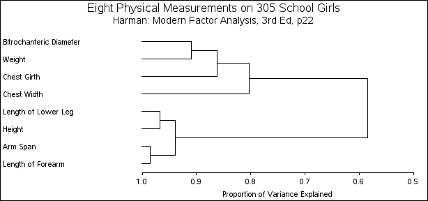
It appears from the diagram that there are two, or possibly three, clusters present. However, the MAXC=8 option forces the VARCLUS procedure to split the clusters until each variable is in its own cluster.
Copyright © 2009 by SAS Institute Inc., Cary, NC, USA. All rights reserved.