| The SEQTEST Procedure |
Example 78.1 Testing the Difference between Two Proportions
This example demonstrates group sequential tests that use an O’Brien-Fleming group sequential design. A clinic is studying the effect of vitamin C supplements in treating flu symptoms. The study consists of patients in the clinic who have exhibited the first sign of flu symptoms within the last 24 hours. These patients are randomly assigned to either the control group (which receives placebo pills) or the treatment group (which receives large doses of vitamin C supplements). At the end of a five-day period, the flu symptoms of each patient are recorded.
Suppose that you know from past experience that flu symptoms disappear in five days for  of patients who experience flu symptoms. The clinic would like to detect a
  symptom disappearance with a high probability. A test that compares the proportions directly specifies the null hypothesis
 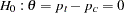 with a one-sided alternative
  and a power of
  at
at  , where
  and
and  are the proportions of symptom disappearance in the treatment group and control group, respectively.
The following statements invoke the SEQDESIGN procedure and request a four-stage group sequential design by using an O’Brien-Fleming method for normally distributed data. The design uses a one-sided alternative hypothesis with early stopping either to accept or reject the null hypothesis  . The BOUNDARYSCALE=MLE option uses the MLE scale to display statistics in the boundary table and boundary plots.
   ods graphics on;
   proc seqdesign altref=0.15
                  boundaryscale=mle
                  ;
      OBrienFleming: design method=obf
                            nstages=4
                            alt=upper
                            stop=both
                            alpha=0.025
                            ;
      samplesize model=twosamplefreq(nullprop=0.6 test=prop);
   ods output Boundary=Bnd_Count;
   run;
   ods graphics off;
The ODS OUTPUT statement with the BOUNDARY=BND_COUNT option creates an output data set named BND_COUNT which contains the resulting boundary information for the subsequent sequential tests.
The "Design Information" table in Output 78.1.1 displays design specifications. With the specified alternative hypothesis , the maximum information is derived to achieve a power of at  . The derived fixed-sample information ratio
  is the maximum information needed for a group sequential design relative to its corresponding fixed-sample design.
| Design Information | |
|---|---|
| Statistic Distribution | Normal |
| Boundary Scale | MLE |
| Alternative Hypothesis | Upper |
| Early Stop | Accept/Reject Null |
| Method | O'Brien-Fleming |
| Boundary Key | Both |
| Alternative Reference | 0.15 |
| Number of Stages | 4 |
| Alpha | 0.025 |
| Beta | 0.1 |
| Power | 0.9 |
| Max Information (Percent of Fixed Sample) | 107.6741 |
| Max Information | 502.8343 |
| Null Ref ASN (Percent of Fixed Sample) | 61.12891 |
| Alt Ref ASN (Percent of Fixed Sample) | 75.89782 |
The "Boundary Information" table in Output 78.1.2 displays the information level, alternative reference, and boundary values at each stage. With the BOUNDARYSCALE=MLE option, the SEQDESIGN procedure displays the output boundaries with the maximum likelihood estimator scale.
| Boundary Information (MLE Scale) Null Reference = 0 |
||||||
|---|---|---|---|---|---|---|
| _Stage_ | Alternative | Boundary Values | ||||
| Information Level | Reference | Upper | ||||
| Proportion | Actual | N | Upper | Beta | Alpha | |
| 1 | 0.2500 | 125.7086 | 107.4808 | 0.15000 | -0.09709 | 0.35291 |
| 2 | 0.5000 | 251.4171 | 214.9617 | 0.15000 | 0.02645 | 0.17645 |
| 3 | 0.7500 | 377.1257 | 322.4425 | 0.15000 | 0.06764 | 0.11764 |
| 4 | 1.0000 | 502.8343 | 429.9233 | 0.15000 | 0.08823 | 0.08823 |
With the specified ODS GRAPHICS ON statement, a detailed boundary plot with the rejection and acceptance regions is displayed by default, as shown in Output 78.1.3. The horizontal axis indicates the information levels for the design. The stages are indicated by vertical lines with accompanying stage numbers. If the test statistic at a stage is in a rejection region, the trial stops and the hypothesis is rejected. If the test statistic is in an acceptance region, then the trial also stops and the hypothesis is accepted. If the statistic is not in a rejection or an acceptance region, the trial continues to the next stage.
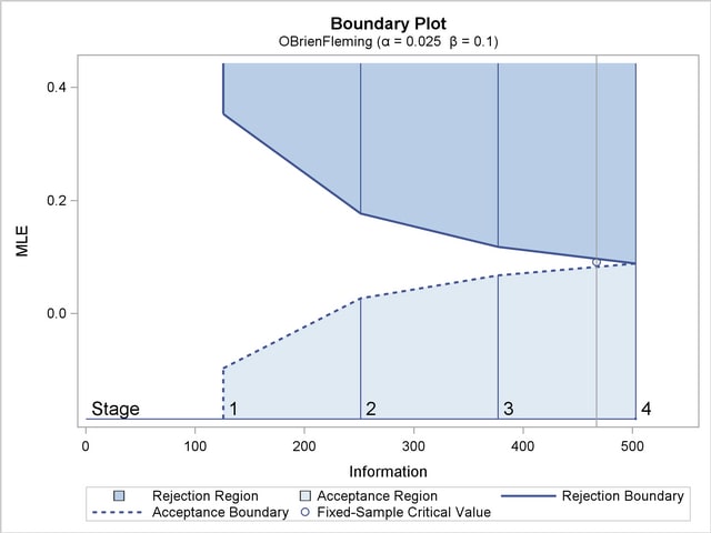
The boundary plot also displays the information level and critical value for the corresponding fixed-sample design. The solid and dashed lines at the fixed-sample information level correspond to the rejection and acceptance lines, respectively.
With the SAMPLESIZE statement, the maximum information is used to derive the required sample size for the study. The "Sample Size Summary" table in Output 78.1.4 displays parameters for the sample size computation.
With the derived maximum information and the specified MODEL= option in the SAMPLESIZE statement, the total sample size in each group for testing the difference between two proportions under the alternative hypothesis is
 |
where  and
and  . By default (or equivalently, if you specify REF=PROP), the required sample sizes are computed under the alternative hypothesis. See the section "Test for the Difference between Two Binomial Proportions" in the chapter "The SEQDESIGN Procedure" for a description of these parameters.
The "Sample Sizes (N)" table in Output 78.1.5 displays the required sample sizes at each stage, in both fractional and integer numbers. The derived sample sizes under the heading Fractional N which correspond to the design are not integers. These sample sizes are rounded up to integers under the heading Ceiling N. In practice, integer sample sizes are used, and the information levels increase slightly. Thus,  ,
,  ,
,  , and
, and  patients are needed in each group for the four stages, respectively.
| Sample Sizes (N) Two-Sample Z Test for Proportion Difference |
||||||||
|---|---|---|---|---|---|---|---|---|
| _Stage_ | Fractional N | Ceiling N | ||||||
| N | N(Grp 1) | N(Grp 2) | Information | N | N(Grp 1) | N(Grp 2) | Information | |
| 1 | 107.48 | 53.74 | 53.74 | 125.7 | 108 | 54 | 54 | 126.3 |
| 2 | 214.96 | 107.48 | 107.48 | 251.4 | 216 | 108 | 108 | 252.6 |
| 3 | 322.44 | 161.22 | 161.22 | 377.1 | 324 | 162 | 162 | 378.9 |
| 4 | 429.92 | 214.96 | 214.96 | 502.8 | 430 | 215 | 215 | 502.9 |
Suppose the trial follows the study plan, and patients are available in each group at stage  . The data set count_1 contains these patients. Output 78.1.6 lists the first
  observations of the data set.
The Trt variable is a grouping variable with value  for a patient in the placebo control group and value for a patient in the treatment group who is given vitamin C supplements. The Resp variable is an indicator variable with value for a patient without flu symptoms after five days and value for a patient with flu symptoms after five days.
The following statements use the GENMOD procedure to estimate the treatment effect at stage :
   proc genmod data=count_1;
      model Resp= Trt;
   ods output ParameterEstimates=Parms_Count1;
   run;
Output 78.1.7 displays the treatment effect at stage .
| Analysis Of Maximum Likelihood Parameter Estimates | |||||||
|---|---|---|---|---|---|---|---|
| Parameter | DF | Estimate | Standard Error | Wald 95% Confidence Limits | Wald Chi-Square | Pr > ChiSq | |
| Intercept | 1 | 0.6296 | 0.0627 | 0.5066 | 0.7526 | 100.68 | <.0001 |
| Trt | 1 | 0.1111 | 0.0887 | -0.0628 | 0.2850 | 1.57 | 0.2105 |
| Scale | 1 | 0.4611 | 0.0314 | 0.4035 | 0.5269 | ||
| Note: | The scale parameter was estimated by maximum likelihood. |
The test statistic is  , and its associated standard error is
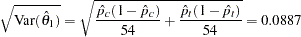 |
The following statements create and display (in Output 78.1.8) the data set that contains the parameter estimate at stage ,  , and its associated standard error
  which are used in the SEQTEST procedure:
   data Parms_Count1;
      set Parms_Count1;
      if Parameter='Trt';
      _Scale_='MLE';
      _Stage_= 1;
      keep _Scale_ _Stage_ Parameter Estimate StdErr;
   run;

   proc print data=Parms_Count1;
      title 'Statistics Computed at Stage 1';
   run;
The initial required sample sizes are derived with the proportions  and
and  . If the observed proportions are different from these assumed values, or if the number of available patients is different from the original plan in one of the stages, then the information level that corresponds to the test statistic is estimated from
 |
The following statements invoke the SEQTEST procedure and test for early stopping at stage :
   ods graphics on;
   proc seqtest Boundary=Bnd_Count
                Parms(Testvar=Trt)=Parms_Count1
                errspendmin=0.001
                boundaryscale=mle
                errspend
                plots=errspend
                ;
   ods output Test=Test_Count1;
   run;
   ods graphics off;
The BOUNDARY= option specifies the input data set that provides the boundary information for the trial at stage , which was generated in the SEQDESIGN procedure. The PARMS=PARMS_COUNT1 option specifies the input data set PARMS_COUNT1 that contains the test statistic and its associated standard error at stage , and the TESTVAR=TRT option identifies the test variable TRT in the data set.
The O’Brien-Fleming design is conservative in early stages and might not be desirable in a clinical trial. The ERRSPENDMIN=0.001 option specifies the minimum error spending at each stage to be  , and it might increase the corresponding nominal
  -value in early stages for the trial. The BOUNDARYSCALE=MLE option uses the MLE scale to display test statistics in the boundary table and boundary plots.
The ODS OUTPUT statement with the TEST=TEST_COUNT1 option creates an output data set named TEST_COUNT1 which contains the updated boundary information for the test at stage . The data set also provides the boundary information that is needed for the group sequential test at the next stage.
The "Design Information" table in Output 78.1.9 displays design specifications. The derived statistics, such as the overall  and
and  levels, are derived from the specified maximum information and boundary values in the BOUNDARY= data set. Note that with a minor change in the information level at stage , the power also changes slightly from the original design.
| Design Information | |
|---|---|
| BOUNDARY Data Set | WORK.BND_COUNT |
| Data Set | WORK.PARMS_COUNT1 |
| Statistic Distribution | Normal |
| Boundary Scale | MLE |
| Alternative Hypothesis | Upper |
| Early Stop | Accept/Reject Null |
| Number of Stages | 4 |
| Alpha | 0.025 |
| Beta | 0.10154 |
| Power | 0.89846 |
| Max Information (Percent of Fixed Sample) | 108.2541 |
| Max Information | 502.834283 |
| Null Ref ASN (Percent of Fixed Sample) | 61.13266 |
| Alt Ref ASN (Percent of Fixed Sample) | 73.9393 |
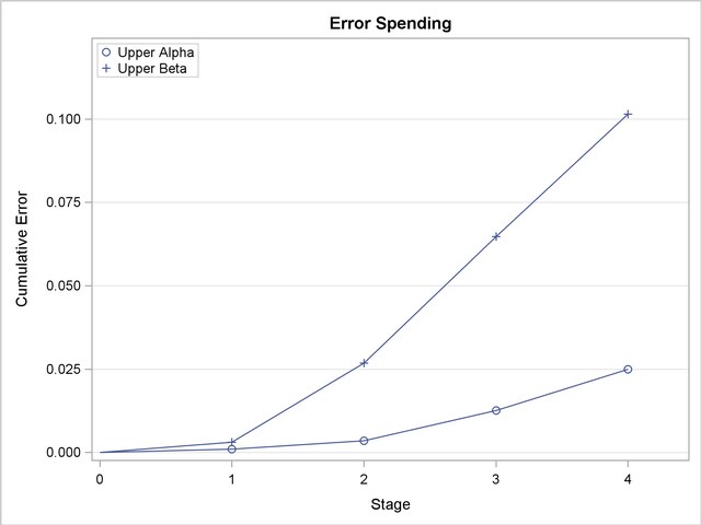
With the ERRSPEND option, the "Error Spending Information" table in Output 78.1.10 displays cumulative error spending at each stage for each boundary. With the default BOUNDARYKEY=ALPHA and the specified ERRSPENDMIN=0.001 options, the spending at each stage is at least .
With the PLOTS=ERRSPEND option, the procedure displays a plot of error spending for each boundary, as shown in Output 78.1.11. The error spending values in the "Error Spending Information" table in Output 78.1.10 are displayed in the plot.
The "Test Information" table in Output 78.1.12 displays the boundary values for the design, test statistic, and resulting action at each stage. With the BOUNDARYSCALE=MLE option, the maximum likelihood estimator scale is used for the test statistic and boundary values. The table shows that the test statistic  is between the upper and boundaries, so the trial continues to the next stage.
| Test Information (MLE Scale) Null Reference = 0 |
|||||||
|---|---|---|---|---|---|---|---|
| _Stage_ | Alternative | Boundary Values | Test | ||||
| Information Level | Reference | Upper | Trt | ||||
| Proportion | Actual | Upper | Beta | Alpha | Estimate | Action | |
| 1 | 0.2525 | 126.9871 | 0.15000 | -0.09304 | 0.27423 | 0.11111 | Continue |
| 2 | 0.5017 | 252.2695 | 0.15000 | 0.02724 | 0.17450 | . | |
| 3 | 0.7508 | 377.5519 | 0.15000 | 0.06813 | 0.11782 | . | |
| 4 | 1.0000 | 502.8343 | 0.15000 | 0.08876 | 0.08876 | . | |
The information level at stage is derived from the standard error,
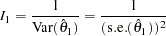 |
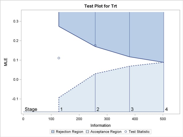
With the default PLOTS=TEST option, the "Test Plot" graph displays boundary values of the design and the test statistic at stage , as shown in Output 78.1.13. It also shows that the observed statistic is in the continuation region.

The observed information level at stage ,  , is slightly larger than the target information level at the design. If an observed information level in the study is substantially different from its target level in the design, then the sample sizes should be adjusted in the subsequent stages to achieve the target information levels.
Suppose the trial continues to the next stage, and patients are available in each group at stage  . The data set COUNT_2 contains these
  patients.
The following statements use the GENMOD procedure to estimate the treatment effect at stage :
   proc genmod data=Count_2;
      model Resp= Trt;
   ods output ParameterEstimates=Parms_Count2;
   run;
The following statements create the parameter estimate at stage ,  , and its associated standard error
  into a test data set:
   data Parms_Count2;
      set Parms_Count2;
      if Parameter='Trt';
      _Scale_='MLE';
      _Stage_= 2;
      keep _Scale_ _Stage_ Parameter Estimate StdErr;
   run;

   proc print data=Parms_Count2;
      title 'Statistics Computed at Stage 2';
   run;
Output 78.1.14 displays the test statistics at stage .
The following statements invoke the SEQTEST procedure and test for early stopping at stage :
   ods graphics on;
   proc seqtest Boundary=Test_Count1
                Parms(Testvar=Trt)=Parms_Count2
                boundaryscale=mle
                ;
   ods output Test=Test_Count2;
   run;
   ods graphics off;
The BOUNDARY= option specifies the input data set that provides the boundary information for the trial at stage , which was generated by the SEQTEST procedure at the previous stage. The PARMS= option specifies the input data set that contains the test statistic and its associated standard error at stage , and the TESTVAR= option identifies the test variable in the data set.
The ODS OUTPUT statement with the TEST=TEST_COUNT2 option creates an output data set named TEST_COUNT2 which contains the updated boundary information for the test at stage . The data set also provides the boundary information that is needed for the group sequential test at the next stage.
The "Test Information" table in Output 78.1.15 displays the boundary values, test statistic, and resulting action at each stage. The table shows that the test statistic  is larger than the corresponding upper alpha boundary value, so the trial stops to reject the hypothesis.
| Test Information (MLE Scale) Null Reference = 0 |
|||||||
|---|---|---|---|---|---|---|---|
| _Stage_ | Alternative | Boundary Values | Test | ||||
| Information Level | Reference | Upper | Trt | ||||
| Proportion | Actual | Upper | Beta | Alpha | Estimate | Action | |
| 1 | 0.2525 | 126.9871 | 0.15000 | -0.09304 | 0.27423 | 0.11111 | Continue |
| 2 | 0.5122 | 257.5571 | 0.15000 | 0.03024 | 0.17001 | 0.17593 | Reject Null |
| 3 | 0.7561 | 380.1957 | 0.15000 | 0.06863 | 0.11722 | . | |
| 4 | 1.0000 | 502.8343 | 0.15000 | 0.08882 | 0.08882 | . | |
With the specified ODS GRAPHICS ON statement, the "Test Plot" is displayed by default, as shown in Output 78.1.16. The plot displays boundary values of the design and the test statistics at the first two stages. As expected, the test statistic at stage is in the "Upper Rejection Region" above the upper alpha boundary.
After a trial is stopped, the "Parameter Estimates" table in Output 78.1.17 displays the stopping stage and the maximum likelihood estimate of the parameter. It also displays the -value, median estimate, and confidence limits for the parameter that correspond to the observed statistic by using the specified sample space ordering.
The MLE statistic at the stopping stage is the maximum likelihood estimate of the parameter and is biased. The computation of -value, unbiased median estimate, and confidence limits depends on the ordering of the sample space  , where
  is the stage number and
  is the observed standardized
  statistic. With the default ORDER=STAGEWISE option, the stagewise ordering that uses counterclockwise ordering around the continuation region is used to compute the -value, unbiased median estimate, and confidence limits. As expected, the -value is less than
  , and the confidence interval does not contain the null reference zero. With the stagewise ordering, the -value is computed as
 |
where  is the observed standardized statistic at stage ,
  is the standardized normal variate at stage ,
  is the standardized normal variate at stage , and
  and
and  are the stage lower and upper rejection boundary values, respectively.
See the section Available Sample Space Orderings in a Sequential Test for a detailed description of the stagewise ordering.
Copyright © 2009 by SAS Institute Inc., Cary, NC, USA. All rights reserved.