| The SEQDESIGN Procedure |
Example 77.12 Creating a Two-Sided Asymmetric Error Spending Design with Early Stopping to Reject or Accept 
This example requests a four-stage two-sided asymmetric group sequential design for normally distributed statistics. The O’Brien-Fleming boundary can be approximated by a gamma family error spending function with parameter  or
or  , and the Pocock boundary can be approximated with parameter
  (Hwang, Shih, and DeCani 1990, p. 1440). The following statements use the gamma error spending function with early stopping to reject or accept the null hypothesis :
   ods graphics on;
   proc seqdesign altref=2
                  pss(cref=0 0.5 1)
                  stopprob(cref=0 1)
                  errspend
                  plots=(asn power errspend)
                  ;
   TwoSidedAsymmetric: design nstages=4
                       method=errfuncgamma(gamma=1)
                       method(beta)=errfuncgamma(gamma=-2)
                       method(upperalpha)=errfuncgamma(gamma=-5)
                       alt=twosided
                       stop=both
                       beta=0.1
                       ;
   run;
   ods graphics off;
The design uses gamma family error spending functions with  for the upper
  boundary, for the lower boundary, and
  for the lower and upper
  boundaries.
The "Design Information" table in Output 77.12.1 displays design specifications and the derived maximum information. Note that in order to attain the same information level for the asymmetric lower and upper boundaries, the derived power at the upper alternative  is larger than the specified
  .
.
| Design Information | |
|---|---|
| Statistic Distribution | Normal |
| Boundary Scale | Standardized Z |
| Alternative Hypothesis | Two-Sided |
| Early Stop | Accept/Reject Null |
| Method | Error Spending |
| Boundary Key | Both |
| Alternative Reference | 2 |
| Number of Stages | 4 |
| Alpha | 0.05 |
| Beta (Lower) | 0.1 |
| Beta (Upper) | 0.06345 |
| Power (Lower) | 0.9 |
| Power (Upper) | 0.93655 |
| Max Information (Percent of Fixed Sample) | 104.0688 |
| Max Information | 3.162386 |
| Null Ref ASN (Percent of Fixed Sample) | 74.16654 |
| Lower Alt Ref ASN (Percent of Fixed Sample) | 59.10271 |
| Upper Alt Ref ASN (Percent of Fixed Sample) | 73.78797 |
The "Method Information" table in Output 77.11.2 displays the specified and error levels and the derived drift parameter. With the same information level used for the asymmetric lower and upper boundaries, only one of the levels is maintained and the other is derived to have the level less than or equal to the specified level.
| Method Information | ||||||
|---|---|---|---|---|---|---|
| Boundary | Method | Alpha | Beta | Error Spending | Alternative Reference |
Drift |
| Function | ||||||
| Upper Alpha | Error Spending | 0.02500 | . | Gamma (Gamma=-5) | 2 | 3.55662 |
| Upper Beta | Error Spending | . | 0.06345 | Gamma (Gamma=-2) | 2 | 3.55662 |
| Lower Beta | Error Spending | . | 0.10000 | Gamma (Gamma=-2) | -2 | -3.55662 |
| Lower Alpha | Error Spending | 0.02500 | . | Gamma (Gamma=1) | -2 | -3.55662 |
With the STOPPROB(CREF=0 1) option, the "Expected Cumulative Stopping Probabilities" table in Output 77.12.3 displays the expected stopping stage and cumulative stopping probabilities at each stage under the null reference  and under the alternative reference
  .
.
| Expected Cumulative Stopping Probabilities Reference = CRef * (Alt Reference) |
|||||||
|---|---|---|---|---|---|---|---|
| CRef | Ref | Expected Stopping Stage |
Source | Stopping Probabilities | |||
| Stage_1 | Stage_2 | Stage_3 | Stage_4 | ||||
| 0.0000 | Lower Alt | 2.851 | Rej Null (Lower Alt) | 0.00875 | 0.01556 | 0.02087 | 0.02500 |
| 0.0000 | Lower Alt | 2.851 | Rej Null (Upper Alt) | 0.00042 | 0.00190 | 0.00704 | 0.02500 |
| 0.0000 | Lower Alt | 2.851 | Reject Null | 0.00917 | 0.01746 | 0.02791 | 0.05000 |
| 0.0000 | Lower Alt | 2.851 | Accept Null | 0.00000 | 0.30125 | 0.79354 | 0.95000 |
| 0.0000 | Lower Alt | 2.851 | Total | 0.00917 | 0.31870 | 0.82145 | 1.00000 |
| 1.0000 | Lower Alt | 2.272 | Rej Null (Lower Alt) | 0.27499 | 0.58934 | 0.79601 | 0.90000 |
| 1.0000 | Lower Alt | 2.272 | Rej Null (Upper Alt) | 0.00000 | 0.00000 | 0.00000 | 0.00000 |
| 1.0000 | Lower Alt | 2.272 | Reject Null | 0.27499 | 0.58934 | 0.79601 | 0.90000 |
| 1.0000 | Lower Alt | 2.272 | Accept Null | 0.00000 | 0.01863 | 0.04935 | 0.10000 |
| 1.0000 | Lower Alt | 2.272 | Total | 0.27499 | 0.60797 | 0.84536 | 1.00000 |
| 0.0000 | Upper Alt | 2.851 | Rej Null (Lower Alt) | 0.00875 | 0.01556 | 0.02087 | 0.02500 |
| 0.0000 | Upper Alt | 2.851 | Rej Null (Upper Alt) | 0.00042 | 0.00190 | 0.00704 | 0.02500 |
| 0.0000 | Upper Alt | 2.851 | Reject Null | 0.00917 | 0.01746 | 0.02791 | 0.05000 |
| 0.0000 | Upper Alt | 2.851 | Accept Null | 0.00000 | 0.30125 | 0.79354 | 0.95000 |
| 0.0000 | Upper Alt | 2.851 | Total | 0.00917 | 0.31870 | 0.82145 | 1.00000 |
| 1.0000 | Upper Alt | 2.836 | Rej Null (Lower Alt) | 0.00002 | 0.00002 | 0.00002 | 0.00002 |
| 1.0000 | Upper Alt | 2.836 | Rej Null (Upper Alt) | 0.05945 | 0.33802 | 0.72323 | 0.93655 |
| 1.0000 | Upper Alt | 2.836 | Reject Null | 0.05947 | 0.33804 | 0.72325 | 0.93657 |
| 1.0000 | Upper Alt | 2.836 | Accept Null | 0.00000 | 0.01182 | 0.03131 | 0.06343 |
| 1.0000 | Upper Alt | 2.836 | Total | 0.05947 | 0.34986 | 0.75456 | 1.00000 |
"Rej Null (Lower Alt)" and "Rej Null (Upper Alt)" under the heading "Source" indicate the probabilities of rejecting the null hypothesis for the lower alternative and for the upper alternative, respectively. "Reject Null" indicates the probability of rejecting the null hypothesis for either the lower or upper alternative, "Accept Null" indicates the probability of accepting the null hypothesis, and "Total" indicates the total probability of stopping the trial.
With the PSS(CREF=0 0.5 1.0) option, the "Power and Expected Sample Sizes" table in Output 77.12.4 displays powers and expected sample sizes under hypothetical references (null hypothesis  ),
),  , and (alternative hypothesis
  ), where
  is the alternative reference. The expected sample sizes are displayed in a scale that indicates a percentage of its corresponding fixed-sample size design.
| Powers and Expected Sample Sizes Reference = CRef * (Alt Reference) |
|||
|---|---|---|---|
| CRef | Ref | Power | Sample Size |
| Percent Fixed-Sample |
|||
| 0.0000 | Lower Alt | 0.02500 | 74.1665 |
| 0.5000 | Lower Alt | 0.34601 | 75.8425 |
| 1.0000 | Lower Alt | 0.90000 | 59.1027 |
| 0.0000 | Upper Alt | 0.02500 | 74.1665 |
| 0.5000 | Upper Alt | 0.41647 | 85.3976 |
| 1.0000 | Upper Alt | 0.93655 | 73.7880 |
Note that at  , the null reference
  , the power with the lower alternative is the lower error
  , and the power with the upper alternative is the upper error . At
  , the alternative reference
  , the power with the lower alternative is the specified power
  , and the power with the upper alternative is greater than the specified power because the same information level is used for these two asymmetric boundaries.
With the PLOTS=POWER option, the procedure displays a plot of the power curves under various hypothetical references, as shown in Output 77.12.5. By default, powers under the lower hypotheses  and under the upper hypotheses
  , are displayed for a two-sided asymmetric design, where
  and
and  and
and  are the lower and upper alternative references, respectively.
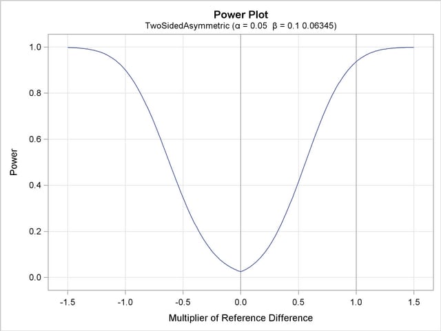
The horizontal axis displays the multiplier of the reference difference. A positive multiplier corresponds to  for the upper alternative hypothesis, and a negative multiplier corresponds to
  for the lower alternative hypothesis. For lower reference hypotheses, the power is the lower error under the null hypothesis () and is under the alternative hypothesis (). For upper reference hypotheses, the power is the upper error under the null hypothesis () and is under the alternative hypothesis ().
With the PLOTS=ASN option, the procedure displays a plot of expected sample sizes under various hypothetical references, as shown in Output 77.12.6. By default, expected sample sizes under the lower hypotheses and under the upper hypotheses are displayed for a two-sided asymmetric design, where and and are the lower and upper alternative references, respectively.
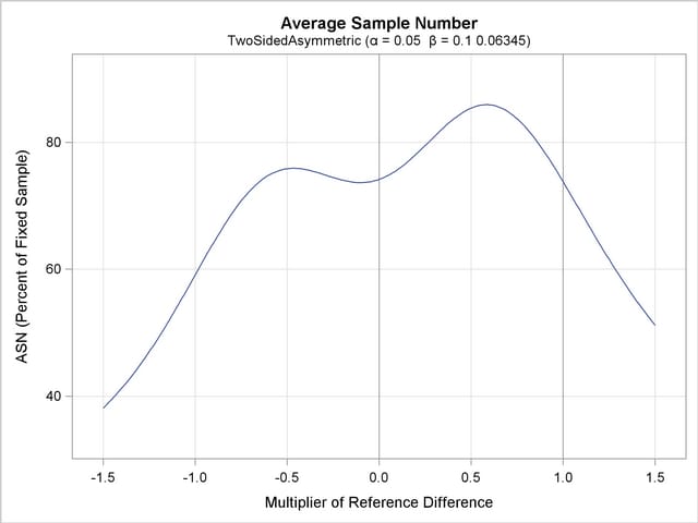
The horizontal axis displays the multiplier of the reference difference. A positive multiplier corresponds to for the upper alternative hypothesis, and a negative multiplier corresponds to for the lower alternative hypothesis.
By default, or when you specify BETAOVERLAP=ADJUST, the SEQDESIGN procedure first derives boundary values without adjusting for the possible overlapping of the two one-sided boundaries based on two corresponding one-sided tests. Then the procedure checks for overlapping of the boundaries at the interim stages. Since the two boundaries overlap at stage  , the boundary values for stage are set to missing, the spending values at stage are set to zero, and the spending values at subsequent stages are adjusted proportionally.
The "Boundary Information" table in Output 77.12.7 displays the information levels, alternative references, and boundary values. The default BOUNDARYSCALE=STDZ option specifies that the standardized  scale be used to display the alternative references and boundary values. The resulting standardized alternative references at stage
  is given by
  , where
  is the specified alternative reference and
  is the information level at stage ,
  .
.
| Boundary Information (Standardized Z Scale) Null Reference = 0 |
||||||||
|---|---|---|---|---|---|---|---|---|
| _Stage_ | Alternative | Boundary Values | ||||||
| Information Level | Reference | Lower | Upper | |||||
| Proportion | Actual | Lower | Upper | Alpha | Beta | Beta | Alpha | |
| 1 | 0.2500 | 0.790597 | -1.77831 | 1.77831 | -2.37610 | . | . | 3.33772 |
| 2 | 0.5000 | 1.581193 | -2.51491 | 2.51491 | -2.35714 | -0.48408 | 0.29400 | 2.94871 |
| 3 | 0.7500 | 2.37179 | -3.08012 | 3.08012 | -2.34861 | -1.36183 | 1.13898 | 2.50473 |
| 4 | 1.0000 | 3.162386 | -3.55662 | 3.55662 | -2.32105 | -2.32105 | 1.95675 | 1.95675 |
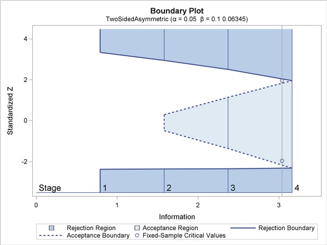
With the specified ODS GRAPHICS ON statement, a detailed boundary plot with the rejection and acceptance regions is displayed by default, as shown in Output 77.12.8.
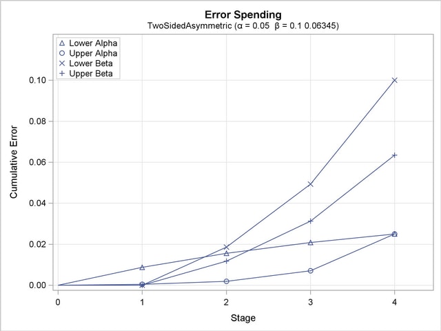
The "Error Spending Information" in Output 77.12.9 displays the cumulative error spending at each stage for each boundary.
With the boundary values missing at stage , there is no early stopping to accept at stage , and the corresponding spending at stage is computed from the rejection region. For example, the upper spending at stage ( ) is the probability of rejecting for the lower alternative under the upper alternative reference.
With the PLOTS=ERRSPEND option, the procedure displays a plot of the cumulative error spending on each boundary at each stage, as shown in Output 77.12.10.
Copyright © 2009 by SAS Institute Inc., Cary, NC, USA. All rights reserved.