| The ROBUSTREG Procedure |
Example 74.3 Growth Study of De Long and Summers
Robust regression and outlier detection techniques have considerable applications to econometrics. The following example from Zaman, Rousseeuw, and Orhan (2001) shows how these techniques substantially improve the ordinary least squares (OLS) results for the growth study of De Long and Summers.
De Long and Summers (1991) studied the national growth of 61 countries from 1960 to 1985 by using OLS with the following data set growth.
   data growth;
      input country$ GDP LFG EQP NEQ GAP @@;
   datalines;
   Argentin  0.0089 0.0118 0.0214 0.2286 0.6079
   Austria   0.0332 0.0014 0.0991 0.1349 0.5809
   Belgium   0.0256 0.0061 0.0684 0.1653 0.4109
   Bolivia   0.0124 0.0209 0.0167 0.1133 0.8634
   Botswana  0.0676 0.0239 0.1310 0.1490 0.9474
   Brazil    0.0437 0.0306 0.0646 0.1588 0.8498
   Cameroon  0.0458 0.0169 0.0415 0.0885 0.9333
   Canada    0.0169 0.0261 0.0771 0.1529 0.1783
   Chile     0.0021 0.0216 0.0154 0.2846 0.5402
   Colombia  0.0239 0.0266 0.0229 0.1553 0.7695
   CostaRic  0.0121 0.0354 0.0433 0.1067 0.7043
   Denmark   0.0187 0.0115 0.0688 0.1834 0.4079
   Dominica  0.0199 0.0280 0.0321 0.1379 0.8293
   Ecuador   0.0283 0.0274 0.0303 0.2097 0.8205
   ElSalvad  0.0046 0.0316 0.0223 0.0577 0.8414
   Ethiopia  0.0094 0.0206 0.0212 0.0288 0.9805
   Finland   0.0301 0.0083 0.1206 0.2494 0.5589
   France    0.0292 0.0089 0.0879 0.1767 0.4708
   Germany   0.0259 0.0047 0.0890 0.1885 0.4585
   Greece    0.0446 0.0044 0.0655 0.2245 0.7924
   Guatemal  0.0149 0.0242 0.0384 0.0516 0.7885
   Honduras  0.0148 0.0303 0.0446 0.0954 0.8850
   HongKong  0.0484 0.0359 0.0767 0.1233 0.7471
   India     0.0115 0.0170 0.0278 0.1448 0.9356
   Indonesi  0.0345 0.0213 0.0221 0.1179 0.9243
   Ireland   0.0288 0.0081 0.0814 0.1879 0.6457
   Israel    0.0452 0.0305 0.1112 0.1788 0.6816
   Italy     0.0362 0.0038 0.0683 0.1790 0.5441
   IvoryCoa  0.0278 0.0274 0.0243 0.0957 0.9207
   Jamaica   0.0055 0.0201 0.0609 0.1455 0.8229
   Japan     0.0535 0.0117 0.1223 0.2464 0.7484
   Kenya     0.0146 0.0346 0.0462 0.1268 0.9415
   Korea     0.0479 0.0282 0.0557 0.1842 0.8807
   Luxembou  0.0236 0.0064 0.0711 0.1944 0.2863
   Madagasc -0.0102 0.0203 0.0219 0.0481 0.9217
   Malawi    0.0153 0.0226 0.0361 0.0935 0.9628
   Malaysia  0.0332 0.0316 0.0446 0.1878 0.7853
   Mali      0.0044 0.0184 0.0433 0.0267 0.9478
   Mexico    0.0198 0.0349 0.0273 0.1687 0.5921
   Morocco   0.0243 0.0281 0.0260 0.0540 0.8405
   Netherla  0.0231 0.0146 0.0778 0.1781 0.3605
   Nigeria  -0.0047 0.0283 0.0358 0.0842 0.8579
   Norway    0.0260 0.0150 0.0701 0.2199 0.3755
   Pakistan  0.0295 0.0258 0.0263 0.0880 0.9180
   Panama    0.0295 0.0279 0.0388 0.2212 0.8015
   Paraguay  0.0261 0.0299 0.0189 0.1011 0.8458
   Peru      0.0107 0.0271 0.0267 0.0933 0.7406
   Philippi  0.0179 0.0253 0.0445 0.0974 0.8747
   Portugal  0.0318 0.0118 0.0729 0.1571 0.8033
   Senegal  -0.0011 0.0274 0.0193 0.0807 0.8884
   Spain     0.0373 0.0069 0.0397 0.1305 0.6613
   SriLanka  0.0137 0.0207 0.0138 0.1352 0.8555
   Tanzania  0.0184 0.0276 0.0860 0.0940 0.9762
   Thailand  0.0341 0.0278 0.0395 0.1412 0.9174
   Tunisia   0.0279 0.0256 0.0428 0.0972 0.7838
   U.K.      0.0189 0.0048 0.0694 0.1132 0.4307
   U.S.      0.0133 0.0189 0.0762 0.1356 0.0000
   Uruguay   0.0041 0.0052 0.0155 0.1154 0.5782
   Venezuel  0.0120 0.0378 0.0340 0.0760 0.4974
   Zambia   -0.0110 0.0275 0.0702 0.2012 0.8695
   Zimbabwe  0.0110 0.0309 0.0843 0.1257 0.8875
   ;
The regression equation they used is
 |
where the response variable is the growth in gross domestic product per worker ( ) and the regressors are labor force growth (
 ), relative GDP gap (
 ), equipment investment (
 ), and nonequipment investment (
 ).
).
The following statements invoke the REG procedure ( Chapter 73, The REG Procedure ) for the OLS analysis:
   proc reg data=growth;
      model GDP  = LFG GAP EQP NEQ ;
   run;
| Parameter Estimates | |||||
|---|---|---|---|---|---|
| Variable | DF | Parameter Estimate |
Standard Error |
t Value | Pr > |t| |
| Intercept | 1 | -0.01430 | 0.01028 | -1.39 | 0.1697 |
| LFG | 1 | -0.02981 | 0.19838 | -0.15 | 0.8811 |
| GAP | 1 | 0.02026 | 0.00917 | 2.21 | 0.0313 |
| EQP | 1 | 0.26538 | 0.06529 | 4.06 | 0.0002 |
| NEQ | 1 | 0.06236 | 0.03482 | 1.79 | 0.0787 |
The OLS analysis shown in Output 74.3.1 indicates that and have a significant influence on at the  level.
The following statements invoke the ROBUSTREG procedure with the default M estimation.
   ods graphics on;

   proc robustreg data=growth plots=all;
      model GDP  = LFG GAP EQP NEQ / diagnostics leverage;
      id country;
   run;

   ods graphics off;
Output 74.3.2 displays model information and summary statistics for variables in the model.
| Model Information | |
|---|---|
| Data Set | WORK.GROWTH |
| Dependent Variable | GDP |
| Number of Independent Variables | 4 |
| Number of Observations | 61 |
| Method | M Estimation |
| Summary Statistics | ||||||
|---|---|---|---|---|---|---|
| Variable | Q1 | Median | Q3 | Mean | Standard Deviation |
MAD |
| LFG | 0.0118 | 0.0239 | 0.0281 | 0.0211 | 0.00979 | 0.00949 |
| GAP | 0.5796 | 0.8015 | 0.8863 | 0.7258 | 0.2181 | 0.1778 |
| EQP | 0.0265 | 0.0433 | 0.0720 | 0.0523 | 0.0296 | 0.0325 |
| NEQ | 0.0956 | 0.1356 | 0.1812 | 0.1399 | 0.0570 | 0.0624 |
| GDP | 0.0121 | 0.0231 | 0.0310 | 0.0224 | 0.0155 | 0.0150 |
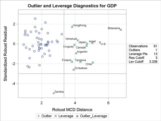
Output 74.3.3 displays the M estimates. Besides and , the robust analysis also indicates that is significant. This new finding is explained by Output 74.3.4, which shows that Zambia, the 60th country in the data, is an outlier. Output 74.3.4 also identifies leverage points based on the robust MCD distances; however, there are no serious high-leverage points in this data set.
| Parameter Estimates | |||||||
|---|---|---|---|---|---|---|---|
| Parameter | DF | Estimate | Standard Error | 95% Confidence Limits | Chi-Square | Pr > ChiSq | |
| Intercept | 1 | -0.0247 | 0.0097 | -0.0437 | -0.0058 | 6.53 | 0.0106 |
| LFG | 1 | 0.1040 | 0.1867 | -0.2619 | 0.4699 | 0.31 | 0.5775 |
| GAP | 1 | 0.0250 | 0.0086 | 0.0080 | 0.0419 | 8.36 | 0.0038 |
| EQP | 1 | 0.2968 | 0.0614 | 0.1764 | 0.4172 | 23.33 | <.0001 |
| NEQ | 1 | 0.0885 | 0.0328 | 0.0242 | 0.1527 | 7.29 | 0.0069 |
| Scale | 1 | 0.0099 | |||||
| Diagnostics | ||||||
|---|---|---|---|---|---|---|
| Obs | country | Mahalanobis Distance | Robust MCD Distance | Leverage | Standardized Robust Residual |
Outlier |
| 1 | Argentin | 2.6083 | 4.0639 | * | -0.9424 | |
| 5 | Botswana | 3.4351 | 6.7391 | * | 1.4200 | |
| 8 | Canada | 3.1876 | 4.6843 | * | -0.1972 | |
| 9 | Chile | 3.6752 | 5.0599 | * | -1.8784 | |
| 17 | Finland | 2.6024 | 3.8186 | * | -1.7971 | |
| 23 | HongKong | 2.1225 | 3.8238 | * | 1.7161 | |
| 27 | Israel | 2.6461 | 5.0336 | * | 0.0909 | |
| 31 | Japan | 2.9179 | 4.7140 | * | 0.0216 | |
| 53 | Tanzania | 2.2600 | 4.3193 | * | -1.8082 | |
| 57 | U.S. | 3.8701 | 5.4874 | * | 0.1448 | |
| 58 | Uruguay | 2.5953 | 3.9671 | * | -0.0978 | |
| 59 | Venezuel | 2.9239 | 4.1663 | * | 0.3573 | |
| 60 | Zambia | 1.8562 | 2.7135 | -4.9798 | * | |
| 61 | Zimbabwe | 1.9634 | 3.9128 | * | -2.5959 | |
Figure 74.3.5 displays robust versions of goodness-of-fit statistics for the model.
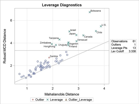
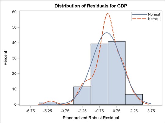
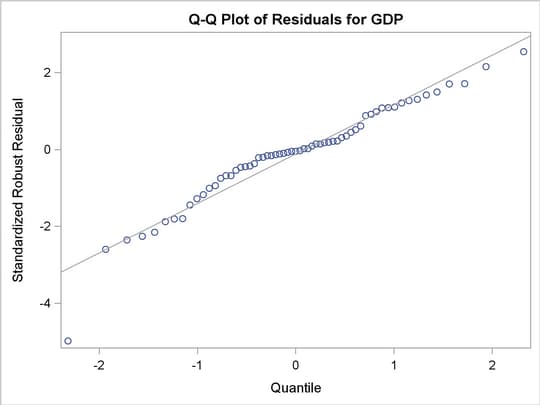
The PLOTS=ALL option generates four diagnostic plots. Figure 74.3.6 and Figure 74.3.7 are for outlier and leverage-point diagnostics. Figure 74.3.8 and Figure 74.3.9 are a histogram and a Q-Q plot of the standardized robust residuals, respectively.
The following statements invoke the ROBUSTREG procedure with LTS estimation, which was used by Zaman, Rousseeuw, and Orhan (2001). The results are consistent with those of M estimation.
   proc robustreg method=lts(h=33) fwls data=growth;
      model GDP  = LFG GAP EQP NEQ / diagnostics leverage ;
      id country;
   run;
| LTS Parameter Estimates | ||
|---|---|---|
| Parameter | DF | Estimate |
| Intercept | 1 | -0.0249 |
| LFG | 1 | 0.1123 |
| GAP | 1 | 0.0214 |
| EQP | 1 | 0.2669 |
| NEQ | 1 | 0.1110 |
| Scale (sLTS) | 0 | 0.0076 |
| Scale (Wscale) | 0 | 0.0109 |
Output 74.3.10 displays the LTS estimates.
| Diagnostics | ||||||
|---|---|---|---|---|---|---|
| Obs | country | Mahalanobis Distance | Robust MCD Distance | Leverage | Standardized Robust Residual |
Outlier |
| 1 | Argentin | 2.6083 | 4.0639 | * | -1.0715 | |
| 5 | Botswana | 3.4351 | 6.7391 | * | 1.6574 | |
| 8 | Canada | 3.1876 | 4.6843 | * | -0.2324 | |
| 9 | Chile | 3.6752 | 5.0599 | * | -2.0896 | |
| 17 | Finland | 2.6024 | 3.8186 | * | -1.6367 | |
| 23 | HongKong | 2.1225 | 3.8238 | * | 1.7570 | |
| 27 | Israel | 2.6461 | 5.0336 | * | 0.2334 | |
| 31 | Japan | 2.9179 | 4.7140 | * | 0.0971 | |
| 53 | Tanzania | 2.2600 | 4.3193 | * | -1.2978 | |
| 57 | U.S. | 3.8701 | 5.4874 | * | 0.0605 | |
| 58 | Uruguay | 2.5953 | 3.9671 | * | -0.0857 | |
| 59 | Venezuel | 2.9239 | 4.1663 | * | 0.4113 | |
| 60 | Zambia | 1.8562 | 2.7135 | -4.4984 | * | |
| 61 | Zimbabwe | 1.9634 | 3.9128 | * | -2.1201 | |
Output 74.3.11 displays outlier and leverage-point diagnostics based on the LTS estimates.
| Parameter Estimates for Final Weighted Least Squares Fit | |||||||
|---|---|---|---|---|---|---|---|
| Parameter | DF | Estimate | Standard Error | 95% Confidence Limits | Chi-Square | Pr > ChiSq | |
| Intercept | 1 | -0.0222 | 0.0093 | -0.0405 | -0.0039 | 5.65 | 0.0175 |
| LFG | 1 | 0.0446 | 0.1771 | -0.3026 | 0.3917 | 0.06 | 0.8013 |
| GAP | 1 | 0.0245 | 0.0082 | 0.0084 | 0.0406 | 8.89 | 0.0029 |
| EQP | 1 | 0.2824 | 0.0581 | 0.1685 | 0.3964 | 23.60 | <.0001 |
| NEQ | 1 | 0.0849 | 0.0314 | 0.0233 | 0.1465 | 7.30 | 0.0069 |
| Scale | 0 | 0.0116 | |||||
Output 74.3.12 displays the final weighted least squares estimates, which are identical to those reported in Zaman, Rousseeuw, and Orhan (2001).
Copyright © 2009 by SAS Institute Inc., Cary, NC, USA. All rights reserved.