| The PRINCOMP Procedure |
Example 69.1 Temperatures
This example analyzes mean daily temperatures in selected cities in January and July. Both the raw data and the principal components are plotted to illustrate how principal components are orthogonal rotations of the original variables.
The following statements create the Temperature data set.
   data Temperature;
      length Cityid $ 2;
      title 'Mean Temperature in January and July for Selected Cities ';
      input City $1-15 January July;
      Cityid = substr(City,1,2);
      datalines;
   Mobile          51.2 81.6
   Phoenix         51.2 91.2
   Little Rock     39.5 81.4
   Sacramento      45.1 75.2
   Denver          29.9 73.0
   Hartford        24.8 72.7
   Wilmington      32.0 75.8
   Washington DC   35.6 78.7
   Jacksonville    54.6 81.0
   Miami           67.2 82.3
   Atlanta         42.4 78.0
   Boise           29.0 74.5
   Chicago         22.9 71.9
   Peoria          23.8 75.1
   Indianapolis    27.9 75.0
   Des Moines      19.4 75.1
   Wichita         31.3 80.7
   Louisville      33.3 76.9
   New Orleans     52.9 81.9
   Portland, ME    21.5 68.0
   Baltimore       33.4 76.6
   Boston          29.2 73.3
   Detroit         25.5 73.3
   Sault Ste Marie 14.2 63.8
   Duluth           8.5 65.6
   Minneapolis     12.2 71.9
   Jackson         47.1 81.7
   Kansas City     27.8 78.8
   St Louis        31.3 78.6
   Great Falls     20.5 69.3
   Omaha           22.6 77.2
   Reno            31.9 69.3
   Concord         20.6 69.7
   Atlantic City   32.7 75.1
   Albuquerque     35.2 78.7
   Albany          21.5 72.0
   Buffalo         23.7 70.1
   New York        32.2 76.6
   Charlotte       42.1 78.5
   Raleigh         40.5 77.5
   Bismarck         8.2 70.8
   Cincinnati      31.1 75.6
   Cleveland       26.9 71.4
   Columbus        28.4 73.6
   Oklahoma City   36.8 81.5
   Portland, OR    38.1 67.1
   Philadelphia    32.3 76.8
   Pittsburgh      28.1 71.9
   Providence      28.4 72.1
   Columbia        45.4 81.2
   Sioux Falls     14.2 73.3
   Memphis         40.5 79.6
   Nashville       38.3 79.6
   Dallas          44.8 84.8
   El Paso         43.6 82.3
   Houston         52.1 83.3
   Salt Lake City  28.0 76.7
   Burlington      16.8 69.8
   Norfolk         40.5 78.3
   Richmond        37.5 77.9
   Spokane         25.4 69.7
   Charleston, WV  34.5 75.0
   Milwaukee       19.4 69.9
   Cheyenne        26.6 69.1
   ;
The following statements plot the temperature data set. The Cityid variable instead of City is used as a data label in the scatter plot for possible label clashing.
   title 'Mean Temperature in January and July for Selected Cities';
   title2 'Plot of Raw Data';
   proc sgplot data=Temperature;
      scatter x=July y=January / datalabel=Cityid;
   run;
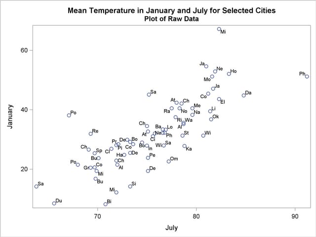
The results are displayed in Output 69.1.1, which shows a scatter diagram of the 64 pairs of data points with July temperatures plotted against January temperatures.
The following statement requests a principal component analysis on the Temperature data set:
   ods graphics on;
   title 'Mean Temperature in January and July for Selected Cities';
   proc princomp data=Temperature cov plots=score(ellipse);
      var July January;
      id Cityid;
   run;
   ods graphics off;
Output 69.1.2 displays the PROC PRINCOMP output. The standard deviation of January (11.712) is higher than the standard deviation of July (5.128). The COV option in the PROC PRINCOMP statement requests the principal components to be computed from the covariance matrix. The total variance is 163.474. The first principal component explains about 94% of the total variance, and the second principal component explains only about 6%. The eigenvalues sum to the total variance.
Note that January receives a higher loading on Prin1 because it has a higher standard deviation than July, and the PRINCOMP procedure calculates the scores by using the centered variables rather than the standardized variables.
| Observations | 64 |
|---|---|
| Variables | 2 |
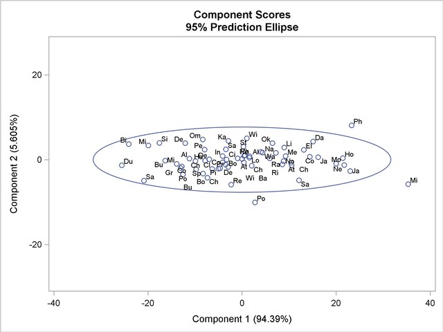
PLOTS=SCORE in the PROC PRINCOMP statement requests a plot of the second principal component against the first principal component as shown in Output 69.1.3. It is clear from this plot that the principal components are orthogonal rotations of the original variables and that the first principal component has a larger variance than the second principal component. In fact, the first component has a larger variance than either of the original variables July and January. The ellipse indicates that Miami, Phoenix, and Portland are possible outliers.
Copyright © 2009 by SAS Institute Inc., Cary, NC, USA. All rights reserved.