| The POWER Procedure |
Example 67.10 Wilcoxon-Mann-Whitney Test
Consider a hypothetical clinical trial to treat interstitial cystitis (IC), a painful, chronic inflammatory condition of the bladder with no known cause that most commonly affects women. Two treatments will be compared: lidocaine alone ("lidocaine") versus lidocaine plus a fictitious experimental drug called Mironel ("Mir+lido"). The design is balanced, randomized, double-blind, and female-only. The primary outcome is a measure of overall improvement at week 4 of the study, measured on a seven-point Likert scale as shown in Table 67.33.
“Compared to when I started |
|
this study, my condition is:” |
|
much worse |
–3 |
worse |
–2 |
slightly worse |
–1 |
the same |
0 |
slightly better |
+1 |
better |
+2 |
much better |
+3 |
The planned data analysis is a one-sided Wilcoxon-Mann-Whitney test with  where the alternative hypothesis represents greater improvement for "Mir+lido."
You are asked to graphically assess the power of the planned trial for sample sizes between 100 and 250, assuming that the conditional outcome probabilities given treatment are equal to the values in Table 67.34.
Response |
|||||||
|---|---|---|---|---|---|---|---|
Treatment |
–3 |
–2 |
–1 |
0 |
+1 |
+2 |
+3 |
lidocaine |
0.01 |
0.04 |
0.20 |
0.50 |
0.20 |
0.04 |
0.01 |
Mir+lido |
0.01 |
0.03 |
0.15 |
0.35 |
0.30 |
0.10 |
0.06 |
Use the following statements to compute the power at sample sizes of 100 and 250 and generate a power curve:
   proc power;
      twosamplewilcoxon
         vardist("lidocaine") = ordinal ((-3 -2 -1 0 1 2 3) :
                                         (.01 .04 .20 .50 .20 .04 .01))
         vardist("Mir+lido") = ordinal ((-3 -2 -1 0 1 2 3) :
                                         (.01 .03 .15 .35 .30 .10 .06))
         variables = "lidocaine" | "Mir+lido"
         sides = u
         ntotal = 100 250
         power = .;
      plot step=10;
   run;
The VARDIST= option is used to define the distribution for each treatment, and the VARIABLES= option specifies the distributions to compare. The SIDES=U option corresponds to the alternative hypothesis that the second distribution ("Mir+lido") is more favorable. The NTOTAL= option specifies the total sample sizes of interest, and the POWER= option with a missing value (.) identifies the parameter to solve for. The default GROUPWEIGHTS= and ALPHA= options specify a balanced design and significance level .
The STEP=10 option in the PLOT statement requests a point for each sample size increment of 10. The default values for the X=, MIN=, and MAX= plot options specify a sample size range of 100 to 250 (the same as in the analysis) for the X axis.
The tabular and graphical results are shown in Output 67.10.1 and Output 67.10.2, respectively.
| Fixed Scenario Elements | |
|---|---|
| Method | O'Brien-Castelloe approximation |
| Number of Sides | U |
| Group 1 Variable | lidocaine |
| Group 2 Variable | Mir+lido |
| Pooled Number of Bins | 7 |
| Alpha | 0.05 |
| Group 1 Weight | 1 |
| Group 2 Weight | 1 |
| NBins Per Group | 1000 |
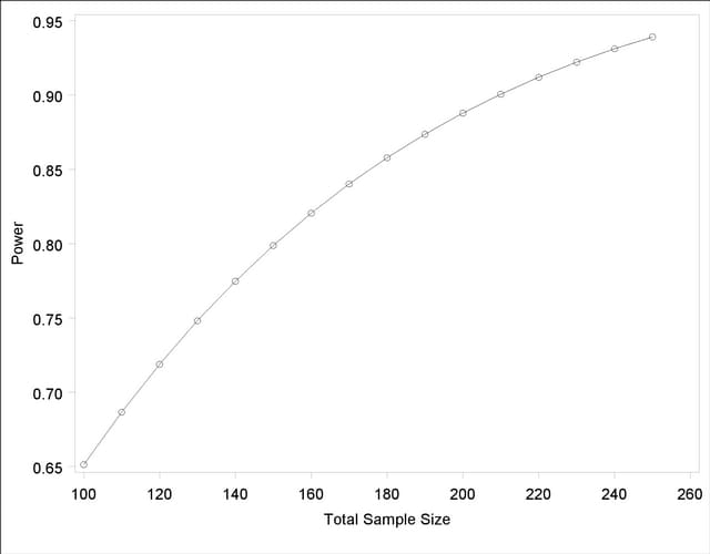
The achieved power ranges from 0.651 to 0.939, increasing with sample size.
Copyright © 2009 by SAS Institute Inc., Cary, NC, USA. All rights reserved.