| The POWER Procedure |
Example 67.4 Noninferiority Test with Lognormal Data
The typical goal in noninferiority testing is to conclude that a new treatment or process or product is not appreciably worse than some standard. This is accomplished by convincingly rejecting a one-sided null hypothesis that the new treatment is appreciably worse than the standard. When designing such studies, investigators must define precisely what constitutes "appreciably worse."
You can use the POWER procedure for sample size analyses for a variety of noninferiority tests, by specifying custom, one-sided null hypotheses for common tests. This example illustrates the strategy (often called Blackwelder’s scheme; Blackwelder 1982) by comparing the means of two independent lognormal samples. The logic applies to one-sample, two-sample, and paired-sample problems involving normally distributed measures and proportions.
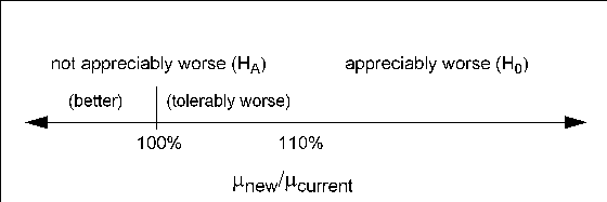
Suppose you are designing a study hoping to show that a new (less expensive) manufacturing process does not produce appreciably more pollution than the current process. Quantifying "appreciably worse" as 10%, you seek to show that the mean pollutant level from the new process is less than 110% of that from the current process. In standard hypothesis testing notation, you seek to reject
 |
in favor of
 |
This is described graphically in Figure 67.8. Mean ratios below 100% are better levels for the new process; a ratio of 100% indicates absolute equivalence; ratios of 100–110% are "tolerably" worse; and ratios exceeding 110% are appreciably worse.
An appropriate test for this situation is the common two-group  test on log-transformed data. The hypotheses become
 |
 |
|||
 |
 |
Measurements of the pollutant level will be taken by using laboratory models of the two processes and will be treated as independent lognormal observations with a coefficient of variation ( ) between 0.5 and 0.6 for both processes. You will end up with 300 measurements for the current process and 180 for the new one. It is important to avoid a Type I error here, so you set the Type I error rate to 0.01. Your theoretical work suggests that the new process will actually reduce the pollutant by about 10% (to 90% of current), but you need to compute and graph the power of the study if the new levels are actually between 70% and 120% of current levels.
Implement the sample size analysis by using the TWOSAMPLEMEANS statement in PROC POWER with the TEST=RATIO option. Indicate power as the result parameter by specifying the POWER= option with a missing value (.). Specify a series of scenarios for the mean ratio between 0.7 and 1.2 by using the MEANRATIO= option. Use the NULLRATIO= option to specify the null mean ratio of 1.10. Specify SIDES=L to indicate a one-sided test with the alternative hypothesis stating that the mean ratio is lower than the null value. Specify the significance level, scenarios for the coefficient of variation, and the group sample sizes by using the ALPHA=, CV=, and GROUPNS= options. Generate a plot of power versus mean ratio by specifying the PLOT statement with the X=EFFECT option to request a plot with mean ratio on the X axis. (The result parameter, here power, is always plotted on the other axis.) Use the STEP= option in the PLOT statement to specify an interval of 0.05 between computed points in the plot.
The following statements perform the desired analysis:
   proc power;
      twosamplemeans test=ratio
         meanratio = 0.7 to 1.2 by 0.1
         nullratio = 1.10
         sides     = L
         alpha     = 0.01
         cv        = 0.5 0.6
         groupns   = (300 180)
         power     = .;
      plot x=effect step=0.05;
   run;
Note the use of SIDES=L, which forces computations for cases that need a rejection region that is opposite to the one providing the most one-tailed power; in this case, it is the lower tail. Such cases will show power that is less than the prescribed Type I error rate. The default option DIST=LOGNORMAL specifies the assumption of lognormally distributed data. The default MIN= and MAX= options in the plot statement specify an X axis range identical to the effect size range in the TWOSAMPLEMEANS statement (mean ratios between 0.7 and 1.2).
Output 67.4.1 and Output 67.4.2 show the results.
| Fixed Scenario Elements | |
|---|---|
| Distribution | Lognormal |
| Method | Exact |
| Number of Sides | L |
| Null Geometric Mean Ratio | 1.1 |
| Alpha | 0.01 |
| Group 1 Sample Size | 300 |
| Group 2 Sample Size | 180 |
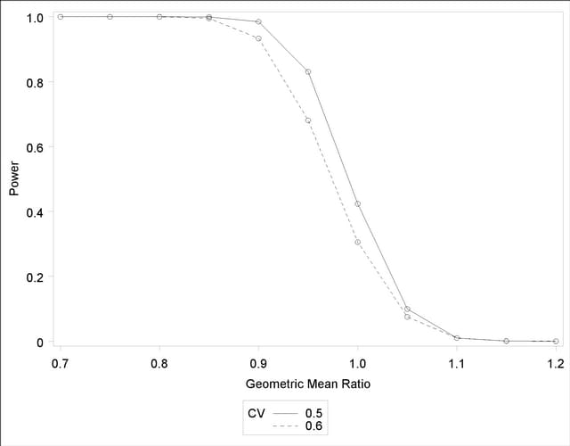
The "Computed Power" table in Output 67.4.1 shows that power exceeds 0.90 if the true mean ratio is 90% or less, as surmised. But power is unacceptably low (0.31–0.42) if the processes happen to be truly equivalent. Note that the power is identical to the alpha level (0.01) if the true mean ratio is 1.10 and below 0.01 if the true mean ratio is appreciably worse (>110%). In Output 67.4.2, the line style identifies the coefficient of variation. The plotting symbols identify locations of actual computed powers; the curves are linear interpolations of these points.
Copyright © 2009 by SAS Institute Inc., Cary, NC, USA. All rights reserved.