Exact Test of a Binomial Proportion (TEST=EXACT)

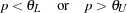
Let be distributed as . The hypotheses for the test of the proportion are as follows:

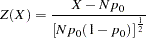
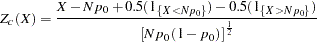
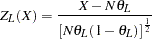
The exact test assumes binomially distributed data and requires and . The test statistic is

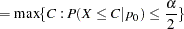
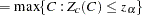
The significance probability is split symmetrically for two-sided tests, in the sense that each tail is filled with as much as possible up to .

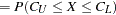
Exact power computations are based on the binomial distribution and computing formulas such as the following from Johnson, Kotz, and Kemp (1992, equation 3.20):

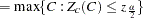
Let and denote lower and upper critical values, respectively. Let denote the achieved (actual) significance level, which for two-sided tests is the sum of the favorable major tail () and the opposite minor tail ().

For the upper one-sided case,

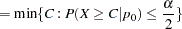
For the lower one-sided case,

For the two-sided case,

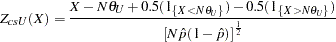
z Test for Binomial Proportion Using Null Variance (TEST=Z VAREST=NULL)

For the normal approximation test, the test statistic is

For the METHOD=EXACT option, the computations are the same as described in the section Exact Test of a Binomial Proportion (TEST=EXACT) except for the definitions of the critical values.

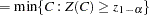
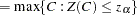
For the upper one-sided case,

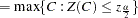
For the lower one-sided case,

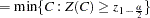
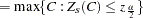
For the two-sided case,

For the METHOD=NORMAL option, the test statistic is assumed to have the normal distribution

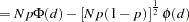
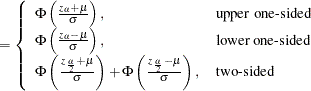
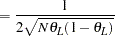
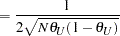
The approximate power is computed as

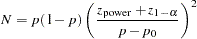
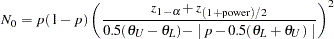
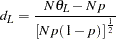
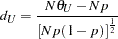
The approximate sample size is computed in closed form for the one-sided cases by inverting the power equation,

and by numerical inversion for the two-sided case.

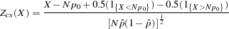
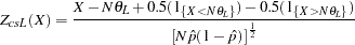
z Test for Binomial Proportion Using Sample Variance (TEST=Z VAREST=SAMPLE)

For the normal approximation test using the sample variance, the test statistic is

where .

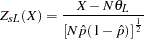
For the METHOD=EXACT option, the computations are the same as described in the section Exact Test of a Binomial Proportion (TEST=EXACT) except for the definitions of the critical values.

For the upper one-sided case,

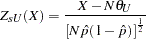
For the lower one-sided case,

For the two-sided case,

For the METHOD=NORMAL option, the test statistic is assumed to have the normal distribution

(see Chow, Shao, and Wang (2003), p. 82).

The approximate power is computed as

The approximate sample size is computed in closed form for the one-sided cases by inverting the power equation,

and by numerical inversion for the two-sided case.

z Test for Binomial Proportion with Continuity Adjustment Using Null Variance (TEST=ADJZ VAREST=NULL)

For the normal approximation test with continuity adjustment, the test statistic is (Pagano and Gauvreau 1993 p. 295):

For the METHOD=EXACT option, the computations are the same as described in the section Exact Test of a Binomial Proportion (TEST=EXACT) except for the definitions of the critical values.

For the upper one-sided case,

For the lower one-sided case,

For the two-sided case,

For the METHOD=NORMAL option, the test statistic is assumed to have the normal distribution , where and are derived as follows.

For convenience of notation, define

Then

and

The probabilities , , and and the truncated expectations and are approximated by assuming the normal-approximate distribution of , . Letting and denote the standard normal PDF and CDF, respectively, and defining as

the terms are computed as follows:

The mean and variance of are thus approximated by

and

The approximate power is computed as

The approximate sample size is computed by numerical inversion.

z Test for Binomial Proportion with Continuity Adjustment Using Sample Variance (TEST=ADJZ VAREST=SAMPLE)

For the normal approximation test with continuity adjustment using the sample variance, the test statistic is

where .

For the METHOD=EXACT option, the computations are the same as described in the section Exact Test of a Binomial Proportion (TEST=EXACT) except for the definitions of the critical values.

For the upper one-sided case,

For the lower one-sided case,

For the two-sided case,

For the METHOD=NORMAL option, the test statistic is assumed to have the normal distribution , where and are derived as follows.

For convenience of notation, define

Then

and

The probabilities , , and and the truncated expectations and are approximated by assuming the normal-approximate distribution of , . Letting and denote the standard normal PDF and CDF, respectively, and defining as

the terms are computed as follows:

The mean and variance of are thus approximated by

and

The approximate power is computed as

The approximate sample size is computed by numerical inversion.

Exact Equivalence Test of a Binomial Proportion (TEST=EQUIV_EXACT)

The hypotheses for the equivalence test are

where and are the lower and upper equivalence bounds, respectively.

The analysis is the two one-sided tests (TOST) procedure as described in Chow, Shao, and Wang (2003) on p. 84, but using exact critical values as on p. 116 instead of normal-based critical values.

Two different hypothesis tests are carried out:

and

If is rejected in favor of and is rejected in favor of , then is rejected in favor of .

The test statistic for each of the two tests ( versus and versus ) is

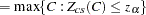
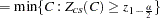
Let denote the critical value of the exact upper one-sided test of versus , and let denote the critical value of the exact lower one-sided test of versus . These critical values are computed in the section Exact Test of a Binomial Proportion (TEST=EXACT). Both of these tests are rejected if and only if . Thus, the exact power of the equivalence test is

The probabilities are computed using Johnson and Kotz (1970, equation 3.20).

z Equivalence Test for Binomial Proportion Using Null Variance (TEST=EQUIV_Z VAREST=NULL)

The hypotheses for the equivalence test are

where and are the lower and upper equivalence bounds, respectively.

The analysis is the two one-sided tests (TOST) procedure as described in Chow, Shao, and Wang (2003) on p. 84, but using the null variance instead of the sample variance.

Two different hypothesis tests are carried out:

and

If is rejected in favor of and is rejected in favor of , then is rejected in favor of .

The test statistic for the test of versus is

The test statistic for the test of versus is

For the METHOD=EXACT option, let denote the critical value of the exact upper one-sided test of versus using . This critical value is computed in the section z Test for Binomial Proportion Using Null Variance (TEST=Z VAREST=NULL). Similarly, let denote the critical value of the exact lower one-sided test of versus using . Both of these tests are rejected if and only if . Thus, the exact power of the equivalence test is

The probabilities are computed using Johnson and Kotz (1970, equation 3.20).

For the METHOD=NORMAL option, the test statistic is assumed to have the normal distribution

and the test statistic is assumed to have the normal distribution

(see Chow, Shao, and Wang (2003), p. 84).

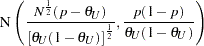
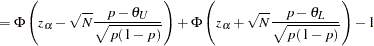
The approximate power is computed as

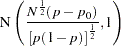
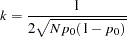
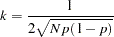
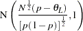
The approximate sample size is computed by numerically inverting the power formula, using the sample size estimate of Chow, Shao, and Wang (2003, p. 85) as an initial guess:

z Equivalence Test for Binomial Proportion Using Sample Variance (TEST=EQUIV_Z VAREST=SAMPLE)

The hypotheses for the equivalence test are

where and are the lower and upper equivalence bounds, respectively.

The analysis is the two one-sided tests (TOST) procedure as described in Chow, Shao, and Wang (2003) on p. 84.

Two different hypothesis tests are carried out:

and

If is rejected in favor of and is rejected in favor of , then is rejected in favor of .

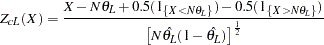
The test statistic for the test of versus is

where .

The test statistic for the test of versus is

For the METHOD=EXACT option, let denote the critical value of the exact upper one-sided test of versus using . This critical value is computed in the section z Test for Binomial Proportion Using Sample Variance (TEST=Z VAREST=SAMPLE). Similarly, let denote the critical value of the exact lower one-sided test of versus using . Both of these tests are rejected if and only if . Thus, the exact power of the equivalence test is

The probabilities are computed using Johnson and Kotz (1970, equation 3.20).

For the METHOD=NORMAL option, the test statistic is assumed to have the normal distribution

and the test statistic is assumed to have the normal distribution

(see Chow, Shao, and Wang (2003), p. 84).

The approximate power is computed as

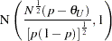
The approximate sample size is computed by numerically inverting the power formula, using the sample size estimate of Chow, Shao, and Wang (2003, p. 85) as an initial guess:

z Equivalence Test for Binomial Proportion with Continuity Adjustment Using Null Variance (TEST=EQUIV_ADJZ VAREST=NULL)

The hypotheses for the equivalence test are

where and are the lower and upper equivalence bounds, respectively.

The analysis is the two one-sided tests (TOST) procedure as described in Chow, Shao, and Wang (2003) on p. 84, but using the null variance instead of the sample variance.

Two different hypothesis tests are carried out:

and

If is rejected in favor of and is rejected in favor of , then is rejected in favor of .

The test statistic for the test of versus is

where .

The test statistic for the test of versus is

For the METHOD=EXACT option, let denote the critical value of the exact upper one-sided test of versus using . This critical value is computed in the section z Test for Binomial Proportion with Continuity Adjustment Using Null Variance (TEST=ADJZ VAREST=NULL). Similarly, let denote the critical value of the exact lower one-sided test of versus using . Both of these tests are rejected if and only if . Thus, the exact power of the equivalence test is

The probabilities are computed using Johnson and Kotz (1970, equation 3.20).

For the METHOD=NORMAL option, the test statistic is assumed to have the normal distribution , and is assumed to have the normal distribution , where , , , and are derived as follows.

For convenience of notation, define

Then

and

The probabilities , , , , , and and the truncated expectations , , , and are approximated by assuming the normal-approximate distribution of , . Letting and denote the standard normal PDF and CDF, respectively, and defining and as

the terms are computed as follows:

The mean and variance of and are thus approximated by

and

The approximate power is computed as

The approximate sample size is computed by numerically inverting the power formula.

z Equivalence Test for Binomial Proportion with Continuity Adjustment Using Sample Variance (TEST=EQUIV_ADJZ VAREST=SAMPLE)

The hypotheses for the equivalence test are

where and are the lower and upper equivalence bounds, respectively.

The analysis is the two one-sided tests (TOST) procedure as described in Chow, Shao, and Wang (2003) on p. 84.

Two different hypothesis tests are carried out:

and

If is rejected in favor of and is rejected in favor of , then is rejected in favor of .

The test statistic for the test of versus is

where .

The test statistic for the test of versus is

For the METHOD=EXACT option, let denote the critical value of the exact upper one-sided test of versus using . This critical value is computed in the section z Test for Binomial Proportion with Continuity Adjustment Using Sample Variance (TEST=ADJZ VAREST=SAMPLE). Similarly, let denote the critical value of the exact lower one-sided test of versus using . Both of these tests are rejected if and only if . Thus, the exact power of the equivalence test is

The probabilities are computed using Johnson and Kotz (1970, equation 3.20).

For the METHOD=NORMAL option, the test statistic is assumed to have the normal distribution , and is assumed to have the normal distribution , where , , and are derived as follows.

For convenience of notation, define

Then

and

The probabilities , , , , , and and the truncated expectations , , , and are approximated by assuming the normal-approximate distribution of , . Letting and denote the standard normal PDF and CDF, respectively, and defining and as

the terms are computed as follows:

The mean and variance of and are thus approximated by

and

The approximate power is computed as

The approximate sample size is computed by numerically inverting the power formula.

Wilson Score Confidence Interval for Binomial Proportion (CI=WILSON)

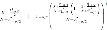
The two-sided % confidence interval for is

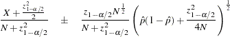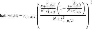
So the half-width for the two-sided % confidence interval is

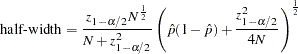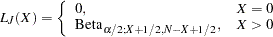
Prob(Width) is calculated exactly by adding up the probabilities of observing each that produces a confidence interval whose half-width is at most a target value :

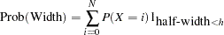For references and more details about this and all other confidence intervals associated with the CI= option, see Binomial Proportion of Chapter 35, The FREQ Procedure.

Agresti-Coull "Add k Successes and Failures" Confidence Interval for Binomial Proportion (CI=AGRESTICOULL)

The two-sided % confidence interval for is

So the half-width for the two-sided % confidence interval is

Prob(Width) is calculated exactly by adding up the probabilities of observing each that produces a confidence interval whose half-width is at most a target value :

Jeffreys Confidence Interval for Binomial Proportion (CI=JEFFREYS)

The two-sided % confidence interval for is

where

and

The half-width of this two-sided % confidence interval is defined as half the width of the full interval:

Prob(Width) is calculated exactly by adding up the probabilities of observing each that produces a confidence interval whose half-width is at most a target value :

Exact Clopper-Pearson Confidence Interval for Binomial Proportion (CI=EXACT)

The two-sided % confidence interval for is

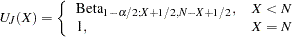
where

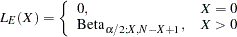and

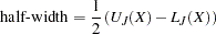
The half-width of this two-sided % confidence interval is defined as half the width of the full interval:

Prob(Width) is calculated exactly by adding up the probabilities of observing each that produces a confidence interval whose half-width is at most a target value :

Wald Confidence Interval for Binomial Proportion (CI=WALD)

The two-sided % confidence interval for is

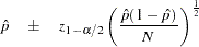So the half-width for the two-sided % confidence interval is

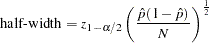Prob(Width) is calculated exactly by adding up the probabilities of observing each that produces a confidence interval whose half-width is at most a target value :

Continuity-Corrected Wald Confidence Interval for Binomial Proportion (CI=WALD_CORRECT)

The two-sided % confidence interval for is

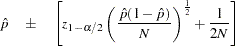So the half-width for the two-sided % confidence interval is

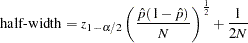Prob(Width) is calculated exactly by adding up the probabilities of observing each that produces a confidence interval whose half-width is at most a target value :