| Statistical Graphics Using ODS |
| Box-Cox Transformation Plot with PROC TRANSREG |
This example is taken from Example 90.2 of Chapter 90, The TRANSREG Procedure. The following statements create a SAS data set that contains failure times for yarn:
   proc format;
      value a -1 =   8 0 =   9 1 =  10;
      value l -1 = 250 0 = 300 1 = 350;
      value o -1 =  40 0 =  45 1 =  50;
   run;

   data yarn;
      input Fail Amplitude Length Load @@;
      format amplitude a. length l. load o.;
      label fail = 'Time in Cycles until Failure';
      datalines;
    674 -1 -1 -1    370 -1 -1  0    292 -1 -1  1    338  0 -1 -1

   ... more lines ...

   ;
The following statements set the output style to JOURNAL2 and run PROC TRANSREG:
   ods listing style=journal2;
   ods graphics on;

   proc transreg data=yarn;
      model BoxCox(fail / convenient lambda=-2 to 2 by 0.05) =
            qpoint(length amplitude load);
   run;
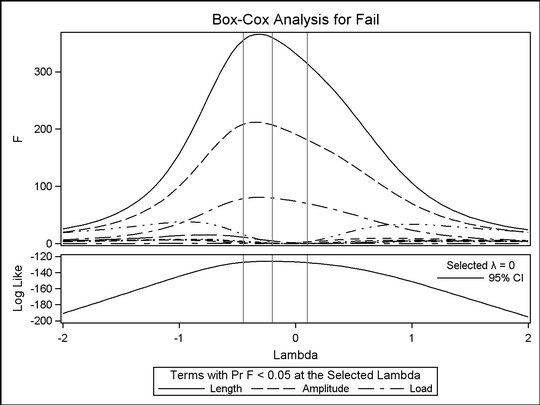
The log-likelihood plot in Figure 21.9 suggests a Box-Cox transformation with  .
.
Figure 21.9
Box-Cox "Significant Effects" Using the JOURNAL2 Style
Copyright © 2009 by SAS Institute Inc., Cary, NC, USA. All rights reserved.