| The NLMIXED Procedure |
| Logistic-Normal Model with Binomial Data |
This example analyzes the data from Beitler and Landis (1985), which represent results from a multi-center clinical trial investigating the effectiveness of two topical cream treatments (active drug, control) in curing an infection. For each of eight clinics, the number of trials and favorable cures are recorded for each treatment. The SAS data set is as follows.
   data infection;
     input clinic t x n;
     datalines;
   1 1 11 36
   1 0 10 37
   2 1 16 20
   2 0 22 32
   3 1 14 19
   3 0  7 19
   4 1  2 16
   4 0  1 17
   5 1  6 17
   5 0  0 12
   6 1  1 11
   6 0  0 10
   7 1  1  5
   7 0  1  9
   8 1  4  6
   8 0  6  7
   ;
Suppose  denotes the number of trials for the
  th clinic and the
  th treatment (
 ), and
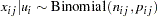
  denotes the corresponding number of favorable cures. Then a reasonable model for the preceding data is the following logistic model with random effects:
 |
and
 |
The notation  indicates the th treatment, and the
  are assumed to be iid
  .
.
The PROC NLMIXED statements to fit this model are as follows:
proc nlmixed data=infection;
parms beta0=-1 beta1=1 s2u=2;
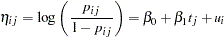
eta = beta0 + beta1*t + u;
expeta = exp(eta);
p = expeta/(1+expeta);
model x ~ binomial(n,p);
random u ~ normal(0,s2u) subject=clinic;
predict eta out=eta;
estimate '1/beta1' 1/beta1;
run;
The PROC NLMIXED statement invokes the procedure, and the PARMS statement defines the parameters and their starting values. The next three statements define  , and the MODEL statement defines the conditional distribution of to be binomial. The RANDOM statement defines u to be the random effect with subjects defined by the clinic variable.
The PREDICT statement constructs predictions for each observation in the input data set. For this example, predictions of  and approximate standard errors of prediction are output to a data set named eta. These predictions include empirical Bayes estimates of the random effects .
The ESTIMATE statement requests an estimate of the reciprocal of  .
.
The output for this model is as follows.
| Specifications | |
|---|---|
| Data Set | WORK.INFECTION |
| Dependent Variable | x |
| Distribution for Dependent Variable | Binomial |
| Random Effects | u |
| Distribution for Random Effects | Normal |
| Subject Variable | clinic |
| Optimization Technique | Dual Quasi-Newton |
| Integration Method | Adaptive Gaussian Quadrature |
The "Specifications" table provides basic information about the nonlinear mixed model (Figure 61.7). For example, the distribution of the response variable, conditional on normally distributed random effects, is binomial. The "Dimensions" table provides counts of various variables. You should check this table to make sure the data set and model have been entered properly. PROC NLMIXED selects five quadrature points to achieve the default accuracy in the likelihood calculations.
The "Parameters" table lists the starting point of the optimization and the negative log likelihood at the starting values (Figure 61.8).
| Iteration History | ||||||
|---|---|---|---|---|---|---|
| Iter | Calls | NegLogLike | Diff | MaxGrad | Slope | |
| 1 | 2 | 37.3622692 | 0.232323 | 2.882077 | -19.3762 | |
| 2 | 3 | 37.1460375 | 0.216232 | 0.921926 | -0.82852 | |
| 3 | 5 | 37.0300936 | 0.115944 | 0.315897 | -0.59175 | |
| 4 | 6 | 37.0223017 | 0.007792 | 0.01906 | -0.01615 | |
| 5 | 7 | 37.0222472 | 0.000054 | 0.001743 | -0.00011 | |
| 6 | 9 | 37.0222466 | 6.57E-7 | 0.000091 | -1.28E-6 | |
| 7 | 11 | 37.0222466 | 5.38E-10 | 2.078E-6 | -1.1E-9 | |
The "Iteration History" table indicates successful convergence in seven iterations (Figure 61.9). The "Fit Statistics" table lists some useful statistics based on the maximized value of the log likelihood.
The "Parameter Estimates" table indicates marginal significance of the two fixed-effects parameters (Figure 61.10). The positive value of the estimate of indicates that the treatment significantly increases the chance of a favorable cure.
The "Additional Estimates" table displays results from the ESTIMATE statement (Figure 61.11). The estimate of  equals
  and its standard error equals
  by the delta method (Billingsley 1986, Cox 1998). Note that this particular approximation produces a
  -statistic identical to that for the estimate of .
Not shown is the eta data set, which contains the original 16 observations and predictions of the .
Copyright © 2009 by SAS Institute Inc., Cary, NC, USA. All rights reserved.