| The MCMC Procedure |
| Posterior Predictive Distribution |
The posterior predictive distribution is the distribution of unobserved observations (prediction) conditional on the observed data. Let  be the observed data,
  be the parameter, and
  be the unobserved data; the posterior predictive distribution is defined to be the following:
 |
 |
 |
|||
 |
|
 |
Given the assumption that the observed and unobserved data are conditional independent given , the posterior predictive distribution can be further simplified as the following:
 |
The posterior predictive distribution is an integral of the likelihood function  with respect to the posterior distribution
  . You can use PROC MCMC to generate samples from a posterior predictive distribution based on draws from the posterior distribution of .
Note that the posterior predictive distribution is not the same as the prior predictive distribution. The prior predictive distribution is  , which is also known as the marginal distribution of the data. The prior predictive distribution is an integral of the likelihood function with respect to the prior distribution:
 |
and the distribution is not conditional on observed data.
You can use the posterior predictive distribution to check whether the model is consistent with data. For more information about using predictive distribution as a model checking tool, see Gelman et al.; 2004, Chapter 6 and the bibliography in that chapter. The idea is to generate replicate data from  —call them
  , for
, for  , where
  is the total number of replicates—compare them to the observed data, and see if there are any large and systematic differences. Large discrepancies suggest possible model misfit. One way to compare the replicate data to the observed data is to first summarize the data to some test quantities, such as the mean, standard deviation, order statistics, and so on. Then compute the tail-area probabilities of the test statistics (based on the observed data) with respect to the estimated posterior predictive distribution using the replicate samples.
Let  denote the function of the test quantity,
  the test quantity using the observed data, and
  the test quantity using the
  th replicate data from the posterior predictive distribution. You calculate the tail-area probability using the following formula:
 |
The following example shows how you can estimate this probability using PROC MCMC.
An Example for Posterior Predictive Distribution
This example uses a normal mixed model to analyze the effects of coaching programs for the scholastic aptitude test (SAT) in eight high schools. For the original analysis of the data, see Rubin (1981). The presentation here follows the analysis and posterior predictive check presented in Gelman et al. (2004). The data are as follows:
   title 'An Example for Posterior Predictive Distribution';

   data SAT;
      input effect se @@;
      ind=_n_;
      datalines;
   28.39 14.9  7.94 10.2 -2.75 16.3
    6.82 11.0 -0.64  9.4  0.63 11.4
   18.01 10.4 12.16 17.6
   ;
The variable effect is the reported test score difference between coached and uncoached students in eight schools. The variable se is the corresponding estimated standard error for that school. In a normal mixed effect model, the variable effect is assumed to be normally distributed:
 |
The parameter  has a normal prior with hyperparameters
  :
:
 |
The hyperprior distribution on  is a uniform prior on the real axis, and the hyperprior distribution on
  is a uniform prior from 0 to infinity.
The following statements fit a normal mixed model, general draws from the posterior predictive distribution, and calculate relevant test quantities.
   ods listing close;
   proc mcmc data=SAT outpost=pred nmc=50000 thin=10 seed=17
      monitor=(yrep mean sd max min);

      array theta[8];
      array yrep[8];
      begincnst;
      call streaminit(1);
      endcnst;

      parms theta: 0;
      parms m 0;
      parms v 1;

      hyper m ~ general(0);
      hyper v ~ general(1,lower=0);
      prior theta: ~ normal(m,var=v);
      mu = theta[ind];
      model effect ~ normal(mu,sd=se);

      /* generate predictive data and calculate test statistics. */
      yrep[ind] = rand('normal', mu, se);
      if (ind eq 8) then do;
         mean = mean(of yrep1-yrep8);
         sd = std(of yrep1-yrep8);
         max = max(of yrep1-yrep8);
         min = min(of yrep1-yrep8);
         end;
      run;
   ods listing;
Four test quantities constructed are: the average (mean), the sample standard deviation (sd), the maximum effect (max), and the minimum effect (min). The MONITOR= option selects yrep (replicate samples) and the four test quantities and saves them to the OUTPOST= data set. The CALL STREAMINIT routine ensures that the RAND function, used here to generate posterior predictive samples, creates a reproducible stream of random numbers. The ODS LISTING CLOSE statement disables listing output because you are primarily interested only in the samples of the monitored quantities. The HYPER, PRIOR, and MODEL statements specify the Bayesian model of interest.
The yrep[ind] assignment statement generates a random normal sample for each predictive observation, indexed by ind, with ind  . Note that this normal distribution is the same as the likelihood function specified in the MODEL statement, with the same mean and standard deviation. To calculate the test quantities, you want to wait until all
  is generated—that is at the last observation of the data set.
The following statements compute the corresponding test statistics, the mean, standard deviation, and the minimum and maximum statistics on the real data and store them in macro variables. You then calculate the tail-area probabilities by counting the number of samples in the data set pred that are greater than the observed test statistics based on the real data.
   proc means data=SAT noprint;
      var effect;
      output out=stat mean=mean max=max min=min stddev=sd;
      run;

   data _null_;
      set stat;
      call symputx('mean',mean);
      call symputx('sd',sd);
      call symputx('min',min);
      call symputx('max',max);
      run;

   data _null_;
      set pred end=eof nobs=nobs;
      ctmean + (mean>&mean);
      ctmin + (min>&min);
      ctmax + (max>&max);
      ctsd + (sd>&sd);
      if eof then do;
         pmean = ctmean/nobs; call symputx('pmean',pmean);
         pmin = ctmin/nobs; call symputx('pmin',pmin);
         pmax = ctmax/nobs; call symputx('pmax',pmax);
         psd = ctsd/nobs; call symputx('psd',psd);
         end;
      run;
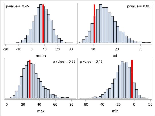
You can plot histograms of each test quantity to visualize the posterior predictive distributions. In addition, you can see where the estimated p-values fall on these densities. Figure 52.12 shows the histograms. To put all four histograms on the same panel, you need to use PROC TEMPLATE (see Chapter 21, Statistical Graphics Using ODS ) and define a new graph template. The following statements defines the template twobytwo:
   proc template;
      define statgraph twobytwo;
         begingraph;
            layout lattice / rows=2 columns=2;
               layout overlay / yaxisopts=(display=none)
                                xaxisopts=(label="mean");
                  layout gridded / columns=2 border=false
                                   autoalign=(topleft topright);
                     entry halign=right "p-value =";
                     entry halign=left eval(strip(put(&pmean, 12.2)));
                  endlayout;
                  histogram mean / binaxis=false;
                  lineparm x=&mean y=0 slope=. /
                           lineattrs=(color=red thickness=5);
               endlayout;
               layout overlay / yaxisopts=(display=none)
                                xaxisopts=(label="sd");
                  layout gridded / columns=2 border=false
                                   autoalign=(topleft topright);
                     entry halign=right "p-value =";
                     entry halign=left eval(strip(put(&psd, 12.2)));
                  endlayout;
                  histogram sd / binaxis=false;
                  lineparm x=&sd y=0 slope=. /
                           lineattrs=(color=red thickness=5);
               endlayout;
               layout overlay / yaxisopts=(display=none)
                                xaxisopts=(label="max");
                  layout gridded / columns=2 border=false
                                   autoalign=(topleft topright);
                     entry halign=right "p-value =";
                     entry halign=left eval(strip(put(&pmax, 12.2)));
                  endlayout;
                  histogram max / binaxis=false;
                  lineparm x=&max y=0 slope=. /
                           lineattrs=(color=red thickness=5);
               endlayout;
               layout overlay / yaxisopts=(display=none)
                                xaxisopts=(label="min");
                  layout gridded / columns=2 border=false
                                   autoalign=(topleft topright);
                     entry halign=right "p-value =";
                     entry halign=left eval(strip(put(&pmin, 12.2)));
                  endlayout;
                  histogram min / binaxis=false;
                  lineparm x=&min y=0 slope=. /
                           lineattrs=(color=red thickness=5);
               endlayout;
            endlayout;
         endgraph;
      end;
   run;
You call PROC SGRENDER (see the SGRENDER procedure in the SAS/GRAPH: Statistical Graphics Procedures Guide) to create the graph, which is shown in Figure 52.12. There are no extreme p-values observed; this supports the notion that the predicted results are similar to the actual observations and that the model fits the data.
   proc sgrender data=pred template=twobytwo;
   run;
Copyright © 2009 by SAS Institute Inc., Cary, NC, USA. All rights reserved.