| The LOGISTIC Procedure |
Example 51.15 Scoring Data Sets with the SCORE Statement
This example first illustrates the syntax used for scoring data sets, then uses a previously scored data set to score a new data set. A generalized logit model is fit to the remote-sensing data set used in the section Linear Discriminant Analysis of Remote-Sensing Data on Crops of Chapter 31, The DISCRIM Procedure, to illustrate discrimination and classification methods. In the following DATA step, the response variable is Crop and the prognostic factors are x1 through x4.
   data Crops;
      length Crop $ 10;
      infile datalines truncover;
      input Crop $ @@;
      do i=1 to 3;
        input x1-x4 @@;
        if (x1 ^= .) then output;
      end;
      input;
      datalines;
   Corn       16 27 31 33  15 23 30 30  16 27 27 26
   Corn       18 20 25 23  15 15 31 32  15 32 32 15
   Corn       12 15 16 73
   Soybeans   20 23 23 25  24 24 25 32  21 25 23 24
   Soybeans   27 45 24 12  12 13 15 42  22 32 31 43
   Cotton     31 32 33 34  29 24 26 28  34 32 28 45
   Cotton     26 25 23 24  53 48 75 26  34 35 25 78
   Sugarbeets 22 23 25 42  25 25 24 26  34 25 16 52
   Sugarbeets 54 23 21 54  25 43 32 15  26 54  2 54
   Clover     12 45 32 54  24 58 25 34  87 54 61 21
   Clover     51 31 31 16  96 48 54 62  31 31 11 11
   Clover     56 13 13 71  32 13 27 32  36 26 54 32
   Clover     53 08 06 54  32 32 62 16
   ;
In the following statements, you specify a SCORE statement to use the fitted model to score the Crops data. The data together with the predicted values are saved in the data set Score1. The output from the PLOTS option is discussed at the end of this section.
   ods graphics on;
   proc logistic data=Crops plots(only)=effect(x=x3);
      model Crop=x1-x4 / link=glogit;
      score out=Score1;
   run;
   ods graphics off;
In the following statements, the model is fit again, the data and the predicted values are saved into the data set Score2, and the OUTMODEL= option saves the fitted model information in the permanent SAS data set sasuser.CropModel:
   proc logistic data=Crops outmodel=sasuser.CropModel;
      model Crop=x1-x4 / link=glogit;
      score data=Crops out=Score2;
   run;
To score data without refitting the model, specify the INMODEL= option to identify a previously saved SAS data set of model information. In the following statements, the model is read from the sasuser.CropModel data set, and the data and the predicted values are saved in the data set Score3. Note that the data set being scored does not have to include the response variable.
   proc logistic inmodel=sasuser.CropModel;
      score data=Crops out=Score3;
   run;
To set prior probabilities on the responses, specify the PRIOR= option to identify a SAS data set containing the response levels and their priors. In the following statements, the Prior data set contains the values of the response variable (because this example uses single-trial MODEL syntax) and a _PRIOR_ variable containing values proportional to the default priors. The data and the predicted values are saved in the data set Score4.
   data Prior;
      length Crop $10.;
      input Crop _PRIOR_;
      datalines;
   Clover     11
   Corn        7
   Cotton      6
   Soybeans    6
   Sugarbeets  6
   ;
   proc logistic inmodel=sasuser.CropModel;
      score data=Crops prior=prior out=Score4 fitstat;
   run;
The "Fit Statistics for SCORE Data" table displayed in Output 51.15.1 shows that 47.22% of the observations are misclassified.
The data sets Score1, Score2, Score3, and Score4 are identical. The following statements display the scoring results in Output 51.15.2:
   proc freq data=Score1;
      table F_Crop*I_Crop / nocol nocum nopercent;
   run;
|
| |||||||||||||||||||||||||||||||||||||||||||||||||||||||||||||||||||||||||||||||||||||||||||||||||||||||||||||||||||||||||||||||||
The following statements use the previously fitted and saved model in the sasuser.CropModel data set to score the observations in a new data set, Test. The results of scoring the test data are saved in the ScoredTest data set and displayed in Output 51.15.3.
   data Test;
      input Crop $ 1-10 x1-x4;
      datalines;
   Corn       16 27 31 33
   Soybeans   21 25 23 24
   Cotton     29 24 26 28
   Sugarbeets 54 23 21 54
   Clover     32 32 62 16
   ;
   proc logistic noprint inmodel=sasuser.CropModel;
      score data=Test out=ScoredTest;
   proc print data=ScoredTest label noobs;
      var F_Crop I_Crop P_Clover P_Corn P_Cotton P_Soybeans P_Sugarbeets;
   run;
| From: Crop | Into: Crop | Predicted Probability: Crop=Clover |
Predicted Probability: Crop=Corn |
Predicted Probability: Crop=Cotton |
Predicted Probability: Crop=Soybeans |
Predicted Probability: Crop=Sugarbeets |
|---|---|---|---|---|---|---|
| Corn | Corn | 0.00342 | 0.90067 | 0.00500 | 0.08675 | 0.00416 |
| Soybeans | Soybeans | 0.04801 | 0.03157 | 0.02865 | 0.82933 | 0.06243 |
| Cotton | Clover | 0.43180 | 0.00015 | 0.21267 | 0.07623 | 0.27914 |
| Sugarbeets | Clover | 0.66681 | 0.00000 | 0.17364 | 0.00000 | 0.15955 |
| Clover | Cotton | 0.41301 | 0.13386 | 0.43649 | 0.00033 | 0.01631 |
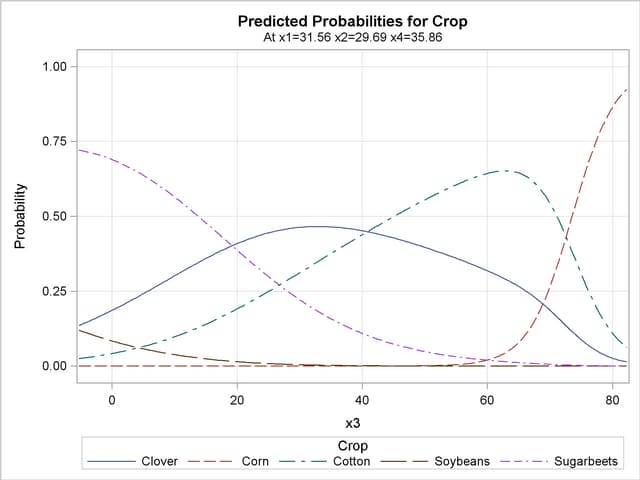
The PLOTS(ONLY)= option specified in the first PROC LOGISTIC invocation produces a plot of the model-predicted probabilities versus X3, holding the other three covariates fixed at their means (Output 51.15.4). This plot shows how the value of X3 affects the probabilities of the various crops when the other prognostic factors are fixed at their means. If you are interested in the effect of X3 when the other covariates are fixed at a certain level—say, 10—specify effect(x=x3 at(x1=10 x2=10 x4=10)).
Copyright © 2009 by SAS Institute Inc., Cary, NC, USA. All rights reserved.