PROC LIFEREG: Modeling Right-Censored Failure Time Data :: SAS/STAT(R) 9.2 User's Guide, Second Edition

The LIFEREG Procedure

Modeling Right-Censored Failure Time Data

The following example demonstrates how you can use the LIFEREG procedure to fit a model to right-censored failure time data.

Suppose you conduct a study of two headache pain relievers. You divide patients into two groups, with each group receiving a different type of pain reliever. You record the time taken (in minutes) for each patient to report headache relief. Because some of the patients never report relief for the entire study, some of the observations are censored.

The following DATA step creates the SAS data set headache:

   data Headache;
      input Minutes Group Censor @@;
      datalines;
   11  1  0   12  1  0   19  1  0   19  1  0
   19  1  0   19  1  0   21  1  0   20  1  0
   21  1  0   21  1  0   20  1  0   21  1  0
   20  1  0   21  1  0   25  1  0   27  1  0
   30  1  0   21  1  1   24  1  1   14  2  0
   16  2  0   16  2  0   21  2  0   21  2  0
   23  2  0   23  2  0   23  2  0   23  2  0
   25  2  1   23  2  0   24  2  0   24  2  0
   26  2  1   32  2  1   30  2  1   30  2  0
   32  2  1   20  2  1
   ;

The data set Headache contains the variable Minutes, which represents the reported time to headache relief; the variable Group, the group to which the patient is assigned; and the variable Censor, a binary variable indicating whether the observation is censored. Valid values of the variable Censor are 0 (no) and 1 (yes). Figure 48.1 shows the first five records of the data set Headache.

Figure 48.1 Headache Data

Obs	Minutes	Group
1	11	1
2	12	1
3	19	1
4	19	1
5	19	1

The following statements invoke the LIFEREG procedure:

   proc lifereg data=Headache;
      class Group;
      model Minutes*Censor(1)=Group;
      output out=New cdf=Prob;
   run;

The CLASS statement specifies the variable Group as the classification variable. The MODEL statement syntax indicates that the response variable Minutes is right censored when the variable Censor takes the value 1. The MODEL statement specifies the variable Group as the single explanatory variable. Because the MODEL statement does not specify the DISTRIBUTION= option, the LIFEREG procedure fits the default type 1 extreme-value distribution by using log(Minutes) as the response. This is equivalent to fitting the Weibull distribution.

The OUTPUT statement creates the output data set New. In addition to containing the variables in the original data set Headache, the SAS data set New also contains the variable Prob. This new variable is created by the CDF= option to contain the estimates of the cumulative distribution function evaluated at the observed response.

The results of this analysis are displayed in the following figures.

Figure 48.2 Model Fitting Information from the LIFEREG Procedure

The LIFEREG Procedure

Model Information
Data Set	WORK.HEADACHE
Dependent Variable	Log(Minutes)
Censoring Variable	Censor
Censoring Value(s)	1
Number of Observations	38
Noncensored Values	30
Right Censored Values	8
Left Censored Values	0
Interval Censored Values	0
Name of Distribution	Weibull
Log Likelihood	-9.37930239

Class Level Information
Name	Levels	Values
Group	2	1 2

Figure 48.2 displays the class level information and model fitting information. There are 30 uncensored observations and 8 right-censored observations. The log likelihood for the Weibull distribution is –9.3793. The log-likelihood value can be used to compare the goodness of fit for different models.

Figure 48.3 Model Parameter Estimates from the LIFEREG Procedure

Analysis of Maximum Likelihood Parameter Estimates
Parameter		DF	Estimate	Standard Error	95% Confidence Limits		Chi-Square	Pr > ChiSq
Intercept		1	3.3091	0.0589	3.1938	3.4245	3161.70	<.0001
Group	1	1	-0.1933	0.0786	-0.3473	-0.0393	6.05	0.0139
Group	2	0	0.0000	.	.	.	.	.
Scale		1	0.2122	0.0304	0.1603	0.2809
Weibull Shape		1	4.7128	0.6742	3.5604	6.2381

The table of parameter estimates is displayed in Figure 48.3. Both the intercept and the slope parameter for the variable group are significantly different from 0 at the 0.05 level. Because the variable group has only one degree of freedom, parameter estimates are given for only one level of the variable group (group=1). However, the estimate for the intercept parameter provides a baseline for group=2.

The resulting model is as follows:

$\text{[math]}$

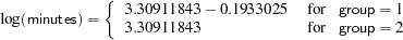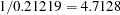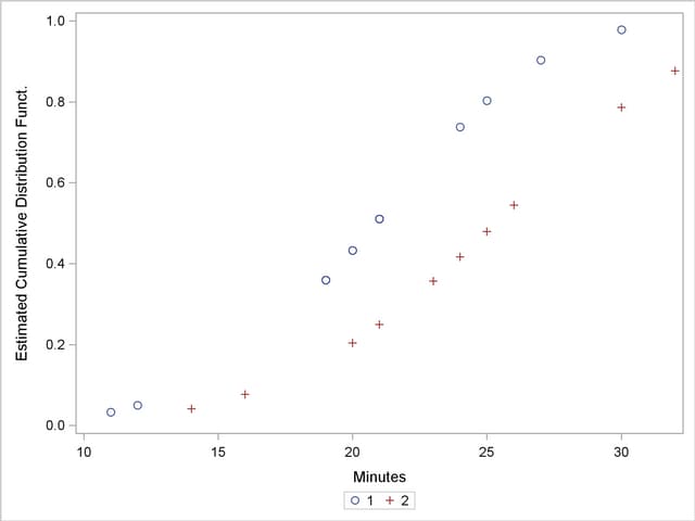
Note that the Weibull shape parameter for this model is the reciprocal of the extreme-value scale parameter estimate shown in Figure 48.3 ( $\text{[math]}$ ).

The following statements produce a graph of the cumulative distribution values versus the variable Minutes.

   proc sgplot data=New;
      scatter x=Minutes y=Prob / group=Group;
      discretelegend;
   run;

Figure 48.4 displays the estimated cumulative distribution function values contained in the output data set New for each group.

Figure 48.4 Plot of the Estimated Cumulative Distribution Function

Top of Page