Example 1

The first example shows that if you can model the direction with the highest sill as a nested model, you then treat the case as a composition of geometric anisotropy and an additional structure that acts only in the direction of the increased sill.

Consider a spatial process where the fitting of theoretical models in your experimental semivariogram produces a correlation structure like the one shown in Figure 46.14. In the direction , the covariance model has a single exponential structure with range and sill . In the direction , the covariance model has two nested structures: an exponential structure with range and sill and a spherical structure with range and sill .

Figure 46.14 Zonal Anisotropy in Two Directions

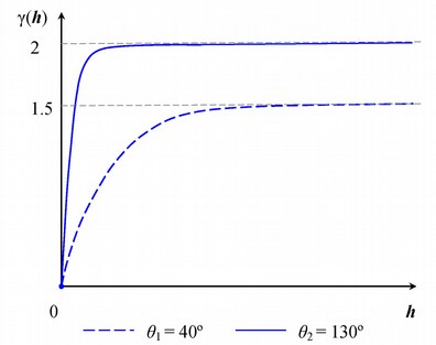
The total sill in the direction of the highest variance is the sum of the nested structures sills . You can consider that your process is characterized: (a) by a geometrically anisotropic exponential structure with common sill across all directions and major axis range and (b) by a spherical structure which is a zonal anisotropy component that contributes only in the direction. Based on the remarks in this section, the RATIO= parameter for the exponential structure is , whereas for the spherical structure you choose a large value, such as .

Then, you can approximate this structure in PROC KRIGE2D by specifying the two structures with the following MODEL statement:

   MODEL FORM=(EXP,SPH) RANGE=(2,1) SCALE=(1.5,0.5)
         ANGLE=(40,130) RATIO=(0.25,1E8);

You can handle more elaborate cases in a similar way, where the covariance models in different directions might all be nested models. Your goal is to model the continuity by starting with a sum of isotropic or geometrically anisotropic structures whose total sill is the lowest sill in all directions. Then, in each of the directions with higher sills you add a zonal anisotropy component in the corresponding sum that compensates for the increased variability in that direction.

Example 2

The second example provides important perspective of the physics in the zonal anisotropy analysis. It is an extreme case of the general guidelines for zonal anisotropy. You examine what happens when each of the directions can be modeled with a simple, nonnested model, and the sills for these models are clearly different.

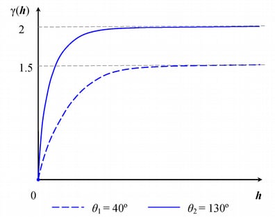
Consider a spatial process with a spatial continuity description almost identical to the one in the previous example. In the direction , the covariance model has again a single exponential structure with range and sill . However, this time in the direction you have fit the experimental semivariogram by using a single exponential structure with range and sill . These models are shown in Figure 46.15.

In this case you have a simplified situation with a single covariance structure in each direction, and neither structure contributes to the sill of the other direction. Hence, you could consider them both to be zonal anisotropy components, where there is no variation due to in the direction and no variation due to in the direction. As a result, both structures can be practically approximated by specifying two models with large RATIO= values. You could then use the following MODEL statement in PROC KRIGE2D to describe the covariance in this example:

   MODEL FORM=(EXP,EXP) RANGE=(2,1) SCALE=(1.5,2)
         ANGLE=(40,130) RATIO=(1E8,1E8);

Figure 46.15 Zonal Anisotropy in Two Directions

However, note that the preceding representation of the spatial continuity accounts only for the specified directions of angles and . Then, the lack of an underlying covariance structure in all other directions can be interpreted as zero continuity everywhere in the process except along the axes at angles and . This would be a very unlikely occurrence in natural processes.

An acceptable alternative would be an attempt to represent the continuity by filling in the intermediate levels of the sill between its lowest and highest values. This would require that you provide zonal anisotropy components for as many directions as possible, thus monitoring closely the spatial continuity by means of the directional change of the process sill. However, in this way you are considering discretized directional intervals, so you are still missing a description for the spatial continuity in the intermediate directions within these intervals. This is also a more complicated approach which can be more tedious than the analysis in the previous example.

For that reason, it is strongly advised that in similar cases you should try to use the analysis illustrated in the previous example. In particular, you should try to model the highest sill direction as a nested structure, such that it comprises a geometrical anisotropy component with cumulative sill equal to the lower sill and a zonal anisotropy component that accounts for the sill difference.