| The GLIMMIX Procedure |
Example 38.10 Multiple Trends Correspond to Multiple Extrema in Profile Likelihoods
The following data set contains observations for a period of 168 months for the "Southern Oscillation Index," measurements of monthly averaged atmospheric pressure differences between Easter Island and Darwin, Australia (Kahaner, Moler, and Nash 1989, Ch. 11.9; National Institute of Standards and Technology 1998). These data are also used as an example in Chapter 50, The LOESS Procedure, in the SAS/STAT User’s Guide.
   data ENSO;
     input Pressure @@;
     Year = _n_ / 12;
   datalines;
    12.9  11.3  10.6  11.2  10.9   7.5   7.7  11.7
    12.9  14.3  10.9  13.7  17.1  14.0  15.3   8.5
     5.7   5.5   7.6   8.6   7.3   7.6  12.7  11.0
    12.7  12.9  13.0  10.9  10.4  10.2   8.0  10.9
    13.6  10.5   9.2  12.4  12.7  13.3  10.1   7.8
     4.8   3.0   2.5   6.3   9.7  11.6   8.6  12.4
    10.5  13.3  10.4   8.1   3.7  10.7   5.1  10.4
    10.9  11.7  11.4  13.7  14.1  14.0  12.5   6.3
     9.6  11.7   5.0  10.8  12.7  10.8  11.8  12.6
    15.7  12.6  14.8   7.8   7.1  11.2   8.1   6.4
     5.2  12.0  10.2  12.7  10.2  14.7  12.2   7.1
     5.7   6.7   3.9   8.5   8.3  10.8  16.7  12.6
    12.5  12.5   9.8   7.2   4.1  10.6  10.1  10.1
    11.9  13.6  16.3  17.6  15.5  16.0  15.2  11.2
    14.3  14.5   8.5  12.0  12.7  11.3  14.5  15.1
    10.4  11.5  13.4   7.5   0.6   0.3   5.5   5.0
     4.6   8.2   9.9   9.2  12.5  10.9   9.9   8.9
     7.6   9.5   8.4  10.7  13.6  13.7  13.7  16.5
    16.8  17.1  15.4   9.5   6.1  10.1   9.3   5.3
    11.2  16.6  15.6  12.0  11.5   8.6  13.8   8.7
     8.6   8.6   8.7  12.8  13.2  14.0  13.4  14.8
   ;
Differences in atmospheric pressure create wind, and the differences recorded in the data set ENSO drive the trade winds in the southern hemisphere. Such time series often do not consist of a single trend or cycle. In this particular case, there are at least two known cycles that reflect the annual weather pattern and a longer cycle that represents the periodic warming of the Pacific Ocean (El Niño).
To estimate the trend in these data by using mixed model technology, you can apply a mixed model smoothing technique such as TYPE=RSMOOTH or TYPE=PSPLINE. The following statements fit a radial smoother to the ENSO data and obtain profile likelihoods for a series of values for the variance of the random spline coefficients:
   data tdata;
     do covp1=0,0.0005,0.05,0.1,0.2,0.5,
              1,2,3,4,5,6,8,10,15,20,50,
              75,100,125,140,150,160,175,
              200,225,250,275,300,350;
        output;
     end;
   run;

   ods select FitStatistics CovParms CovTests;
   proc glimmix data=enso noprofile;
      model pressure = year;
      random year / type=rsmooth knotmethod=equal(50);
      parms (2) (10);
      covtest tdata=tdata / parms;
      ods output covtests=ct;
   run;
The tdata data set contains value for the variance of the radial smoother variance for which the profile likelihood of the model is to be computed. The profile likelihood is obtained by setting the radial smoother variance at the specified value and estimating all other parameters subject to that constraint.
Because the model contains a residual variance and you need to specify nonzero values for the first covariance parameter, the NOPROFILE is added to the PROC GLIMMIX statements. If the residual variance is profiled from the estimation, you cannot fix covariance parameters at a given value, because they would be reexpressed during model fitting in terms of ratios with the profiled (and changing) variance.
The PARMS statement determines starting values for the covariance parameters for fitting the (full) model. The PARMS option in the COVTEST statement requests that the input parameters be added to the output and the output data set. This is useful for subsequent plotting of the profile likelihood function.
The "Fit Statistics" table displays the  restricted log likelihood of the model (
 , Output 38.10.1). The estimate of the variance of the radial smoother coefficients is
  .
.
The "Test of Covariance Parameters" table displays the restricted log likelihood for each observation in the tdata set. Because the tdata data set specifies values for only the first covariance parameter, the second covariance parameter is free to vary and the values for  2 Res Log Like are profile likelihoods. Notice that for a number of values of CovP1 the chi-square statistic is missing in this table. For these values the 2 Res Log Like is smaller than that of the full model. The model did not converge to a global minimum of the negative restricted log likelihood.
| Fit Statistics | |
|---|---|
| -2 Res Log Likelihood | 897.76 |
| AIC (smaller is better) | 901.76 |
| AICC (smaller is better) | 901.83 |
| BIC (smaller is better) | 897.76 |
| CAIC (smaller is better) | 899.76 |
| HQIC (smaller is better) | 897.76 |
| Generalized Chi-Square | 1554.38 |
| Gener. Chi-Square / DF | 9.36 |
| Radial Smoother df(res) | 153.52 |
| Covariance Parameter Estimates | ||
|---|---|---|
| Cov Parm | Estimate | Standard Error |
| Var[RSmooth(Year)] | 3.5719 | 3.7672 |
| Residual | 9.3638 | 1.3014 |
| Tests of Covariance Parameters Based on the Restricted Likelihood |
|||||||
|---|---|---|---|---|---|---|---|
| Label | DF | -2 Res Log Like | ChiSq | Pr > ChiSq | Input Parameters | Note | |
| CovP1 | CovP2 | ||||||
| WORK.TDATA | 1 | 893.01 | . | 1.0000 | 0.0000 | 9.36 | MI |
| WORK.TDATA | 1 | 892.76 | . | 1.0000 | 0.0005 | 9.36 | DF |
| WORK.TDATA | 1 | 897.34 | . | 1.0000 | 0.0500 | 9.36 | DF |
| WORK.TDATA | 1 | 898.53 | 0.77 | 0.3816 | 0.1000 | 9.36 | DF |
| WORK.TDATA | 1 | 899.38 | 1.62 | 0.2038 | 0.2000 | 9.36 | DF |
| WORK.TDATA | 1 | 899.49 | 1.73 | 0.1888 | 0.5000 | 9.36 | DF |
| WORK.TDATA | 1 | 898.83 | 1.07 | 0.3016 | 1.0000 | 9.36 | DF |
| WORK.TDATA | 1 | 898.04 | 0.28 | 0.5967 | 2.0000 | 9.36 | DF |
| WORK.TDATA | 1 | 897.79 | 0.03 | 0.8693 | 3.0000 | 9.36 | DF |
| WORK.TDATA | 1 | 897.77 | 0.01 | 0.9145 | 4.0000 | 9.36 | DF |
| WORK.TDATA | 1 | 897.86 | 0.10 | 0.7517 | 5.0000 | 9.36 | DF |
| WORK.TDATA | 1 | 897.99 | 0.23 | 0.6311 | 6.0000 | 9.36 | DF |
| WORK.TDATA | 1 | 898.27 | 0.51 | 0.4761 | 8.0000 | 9.36 | DF |
| WORK.TDATA | 1 | 898.49 | 0.73 | 0.3919 | 10.0000 | 9.36 | DF |
| WORK.TDATA | 1 | 898.70 | 0.94 | 0.3318 | 15.0000 | 9.36 | DF |
| WORK.TDATA | 1 | 898.45 | 0.69 | 0.4068 | 20.0000 | 9.36 | DF |
| WORK.TDATA | 1 | 892.63 | . | 1.0000 | 50.0000 | 9.36 | DF |
| WORK.TDATA | 1 | 887.44 | . | 1.0000 | 75.0000 | 9.36 | DF |
| WORK.TDATA | 1 | 883.79 | . | 1.0000 | 100.0000 | 9.36 | DF |
| WORK.TDATA | 1 | 881.55 | . | 1.0000 | 125.0000 | 9.36 | DF |
| WORK.TDATA | 1 | 880.72 | . | 1.0000 | 140.0000 | 9.36 | DF |
| WORK.TDATA | 1 | . | . | . | 150.0000 | 9.36 | |
| WORK.TDATA | 1 | 880.07 | . | 1.0000 | 160.0000 | 9.36 | DF |
| WORK.TDATA | 1 | 879.85 | . | 1.0000 | 175.0000 | 9.36 | DF |
| WORK.TDATA | 1 | . | . | . | 200.0000 | 9.36 | |
| WORK.TDATA | 1 | 880.21 | . | 1.0000 | 225.0000 | 9.36 | DF |
| WORK.TDATA | 1 | 880.80 | . | 1.0000 | 250.0000 | 9.36 | DF |
| WORK.TDATA | 1 | 881.56 | . | 1.0000 | 275.0000 | 9.36 | DF |
| WORK.TDATA | 1 | 882.44 | . | 1.0000 | 300.0000 | 9.36 | DF |
| WORK.TDATA | 1 | 884.41 | . | 1.0000 | 350.0000 | 9.36 | DF |
MI: P-value based on a mixture of chi-squares.
The following statements plot the restricted profile log likelihood (Output 38.10.2):
   proc sgplot data=ct;
      series y=objective x=covp1;
   run;
2 Restricted Profile Log Likelihood for Smoothing Variance
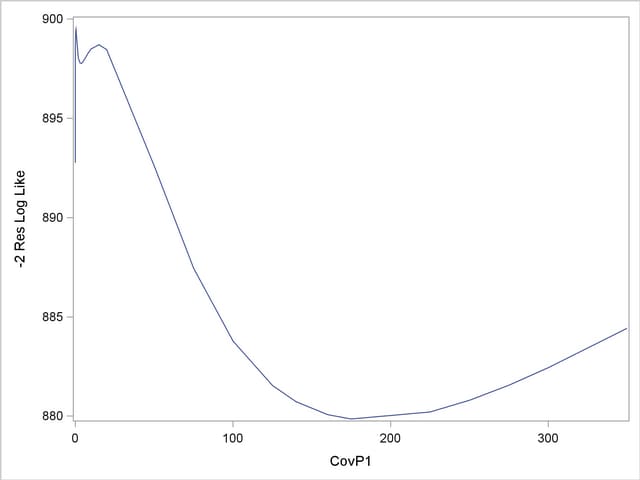
The local minimum at which the optimization stopped is clearly visible, as are a second local minimum near zero and the global minimum near 180.
The observed and predicted pressure differences that correspond to the three minima are shown in Output 38.10.3. These results were produced with the following statements:
   proc glimmix data=enso;
      model pressure = year;
      random year / type=rsmooth knotmethod=equal(50);
      parms (0) (10);
      output out=gmxout1 pred=pred1;
   run;
   proc glimmix data=enso;
      model pressure = year;
      random year / type=rsmooth knotmethod=equal(50);
      output out=gmxout2 pred=pred2;
      parms (2) (10);
   run;
   proc glimmix data=enso;
      model pressure = year;
      random year / type=rsmooth knotmethod=equal(50);
      output out=gmxout3 pred=pred3;
      parms (200) (10);
   run;
   data plotthis; merge gmxout1 gmxout2 gmxout3;
   run;
   proc sgplot data=plotthis;
      scatter x=year y=Pressure;
      series  x=year y=pred1 /
           lineattrs   = (pattern=solid thickness=2)
           legendlabel = "Var[RSmooth] = 0.0005"
           name        = "pred1";
      series  x=year y=pred2 /
           lineattrs   = (pattern=dot thickness=2)
           legendlabel = "Var[RSmooth] = 3.5719"
           name        = "pred2";
      series  x=year y=pred3 /
           lineattrs   = (pattern=dash thickness=2)
           legendlabel = "Var[RSmooth] = 186.71"
           name        = "pred3";
      keylegend "pred1" "pred2" "pred3" / across=2;
   run;
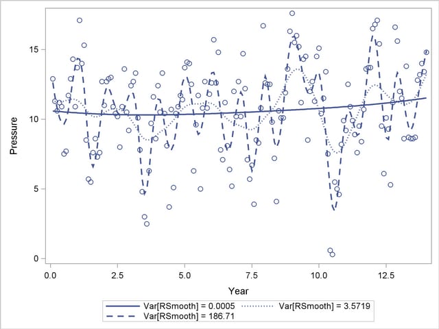
The one-year cycle ( ) and the El Niño cycle (
 ) are clearly visible. Notice that a larger smoother variance results in larger BLUPs and hence larger adjustments to the fixed-effects model. A large smoother variance thus results in a more wiggly fit. The third local minimum at
  applies only very small adjustments to the linear regression between pressure and time, creating slight curvature.
Copyright © 2009 by SAS Institute Inc., Cary, NC, USA. All rights reserved.