The CALIS Procedure

Getting Started: CALIS Procedure

Statements in the CALIS procedure are used for various purposes:

PROC CALIS statement invokes the procedure.
Main model specification statements: LINEQS, RAM, FACTOR, and COSAN. These statements define the model type and specify the main model.
Subsidiary model specification statements: STD, COV, VARNAMES, MATRIX, and PARAMETERS. These statements define additional parameters and model features that supplement to the main model specification. The usage of these statements depends on the model type specified in the main model statement. See the section The Model Type and Related Statements for more details.
Statements for constraining parameters: BOUNDS, LINCON, and NLINCON. The SAS programming statements can also be used to constrain parameters. See the section Constrained Estimation for more details.
General data processing statements: BY, VAR, PARTIAL, FREQ, and WEIGHT. The usages of these statements are common to other SAS procedures.
Other statements: The STRUCTEQ statement is used for defining "structural equations" in the model. The NLOPTIONS statement is used for fine-tuning the optimization techniques for the analysis. The SAS programming statements are used for computing dependent parametric functions that are useful for model specification or setting up constraints in the model.

The Model Type and Related Statements

There are four sets of statements available in the CALIS procedure to specify a model. Each set represents a model type supported by the CALIS procedure. For the LINEQS model with linear equations input, you can specify the following statements:

LINEQS analysis model in equations notation;

STD variance pattern;

COV covariance pattern;

PARAMETERS parameter names from programming statements;

For the RAM model, you can specify the following statements:

RAM analysis model in list notation;

VARNAMES names of latent and error variables;

PARAMETERS parameter names from programming statements;

For the (confirmatory) factor model, you can specify the following statements:

FACTOR options;

MATRIX definition of matrix elements;

VARNAMES names of latent and residual variables;

PARAMETERS parameter names from programming statements;

For the COSAN model, you can specify the following statements:

COSAN analysis model in matrix notation;

MATRIX definition of matrix elements ;

VARNAMES names of additional variables ;

PARAMETERS parameter names from programming statements;

You can also specify a model by using an INRAM= data set, which is usually a version of an OUTRAM= data set produced by a previous PROC CALIS analysis (and possibly modified). If no INRAM= data set is specified, you must use one of the four main model specification statements that defines the analysis model: LINEQS, RAM, FACTOR, or COSAN.

LISREL model input is not directly supported in PROC CALIS. However, with careful constructions you can use either the LINEQS, RAM, or COSAN model input to specify a LISREL model equivalently.

In the following sections, each model type supported by the CALIS procedure is discussed in more details.

LINEQS Model Specification

By using notation similar to that originally developed by Bentler for his EQS program, you can also describe the model by a set of linear equations combined with variance and covariance specifications. The displayed output can be in either equation form or matrix form.

The following statements define the structural model of the alienation example as a LINEQS model:

    lineqs                                           
         V1 =         F1                  + E1,      
         V2 =    .833 F1                  + E2,      
         V3 =         F2                  + E3,      
         V4 =    .833 F2                  + E4,      
         V5 =         F3                  + E5,      
         V6 = Lamb (.5) F3                + E6,      
         F1 = Gam1(-.5) F3                + D1,      
         F2 = Beta (.5) F1 + Gam2(-.5) F3 + D2;      
    std                                              
         E1-E6 = The1-The2 The1-The4 (6 * 3.),       
         D1-D2 = Psi1-Psi2 (2 * 4.),                 
         F3    = Phi (6.) ;                          
    cov                                              
         E1 E3 = The5 (.2),                          
         E4 E2 = The5 (.2);

The LINEQS statement shows the equations in the section LINEQS Model, except that in this case the coefficients to be estimated can be followed (optionally) by the initial value to use in the optimization process. If you do not specify initial values for the parameters in a LINEQS statement, PROC CALIS tries to assign these values automatically. The endogenous variables used on the left side can be manifest variables (with names that must be defined by the input data set) or latent variables (which must have names starting with F). The variables used on the right side can be manifest variables, latent variables (with names that must start with an F), or error variables (which must have names starting with an E or D). Commas separate the equations. The coefficients to be estimated are indicated by names. If no name is used, the coefficient is constant, either equal to a specified number or, if no number is used, equal to 1. The VAR statement in Bentler’s notation is replaced here by the STD statement, because the VAR statement in PROC CALIS defines the subset of manifest variables in the data set to be analyzed. The variable names used in the STD or COV statement must be exogenous (that is, they should not occur on the left side of any equation). The STD and COV statements define the diagonal and off-diagonal elements in the $\text{[math]}$ matrix. The parameter specifications in the STD and COV statements are separated by commas. Using $\text{[math]}$ variable names on the left of an equal sign in a COV statement means that the parameter list on the right side refers to all $\text{[math]}$ distinct variable pairs in the $\text{[math]}$ matrix. Identical coefficient names indicate parameters constrained to be equal. You can also use prefix names to specify those parameters for which you do not need a precise name in any parameter constraint.

See the section LINEQS Model Statement for more information about the precise syntax rules for a LINEQS statement.

RAM Model Specification

The RAM model enables a path diagram to be transcribed into a RAM statement in list form. The displayed output from the RAM statement is in matrix or list form.

The following statement defines the structural model of the alienation example as a RAM model:

   ram                         
        1   1  7  1.       ,   
        1   2  7  .833     ,   
        1   3  8  1.       ,   
        1   4  8  .833     ,   
        1   5  9  1.       ,   
        1   6  9  .5    Lamb , 
        1   7  9  -.5   Gam1 , 
        1   8  7  .5    Beta , 
        1   8  9  -.5   Gam2 , 
        2   1  1  3.    The1 , 
        2   2  2  3.    The2 , 
        2   3  3  3.    The1 , 
        2   4  4  3.    The2 , 
        2   5  5  3.    The3 , 
        2   6  6  3.    The4 , 
        2   1  3  .2    The5 , 
        2   2  4  .2    The5 , 
        2   7  7  4.    Psi1 , 
        2   8  8  4.    Psi2 , 
        2   9  9  6.    Phi ;

You must assign numbers to the nodes in the path diagram. In the path diagram of Figure 25.1, the boxes corresponding to the six manifest variables V1, ..., V6 are assigned the number of the variable in the covariance matrix (1, ..., 6); the circles corresponding to the three latent variables F1, F2, and F3 are given the numbers 7, 8, and 9. The path diagram contains 20 paths between the nine nodes; nine of the paths are one-headed arrows and eleven are two-headed arrows.

The RAM statement contains a list of items separated by commas. Each item corresponds to an arrow in the path diagram. The first entry in each item is the number of arrow heads (matrix number), the second entry shows where the arrow points to (row number), the third entry shows where the arrow comes from (column number), the fourth entry gives the (initial) value of the coefficient, and the fifth entry assigns a name if the path represents a parameter rather than a constant. If you specify the fifth entry as a parameter name, then the fourth list entry can be omitted, since PROC CALIS tries to assign an initial value to this parameter.

See the section RAM Model Statement for more information about the RAM statement.

COSAN Model Specification

You specify the model for a generalized COSAN analysis with a COSAN statement and one or more MATRIX statements. The COSAN statement determines the name, dimension, and type (identity, diagonal, symmetric, upper, lower, general, inverse, and so forth) of each matrix in the model. You can specify the values of the constant elements in each matrix and give names and initial values to the elements that are to be estimated as parameters or functions of parameters by using MATRIX statements. The resulting displayed output is in matrix form.

The following statements define the structural model of the alienation example as a COSAN model:

   cosan J(9, Ide) * A(9, Gen, Imi) * P(9, Sym);
   matrix A
             [ ,7] = 1. .833  5 * 0. Beta (.5) ,
             [ ,8] = 2 * 0.  1.  .833 ,
             [ ,9] = 4 * 0.  1.  Lamb Gam1-Gam2 (.5 2 * -.5);
   matrix P
             [1,1] = The1-The2 The1-The4 (6 * 3.) ,
             [7,7] = Psi1-Psi2 Phi (2 * 4. 6.) ,
             [3,1] = The5 (.2) ,
             [4,2] = The5 (.2) ;

The matrix model specified in the COSAN statement is the RAM model

$\text{[math]}$

with selection matrix $\text{[math]}$ and

$\text{[math]}$

The COSAN statement must contain only the matrices up to the central matrix $\text{[math]}$ because of the symmetry of each matrix term in a COSAN model. Each matrix name is followed by one to three arguments in parentheses. The first argument is the number of columns. The second and third arguments are optional, and they specify the form of the matrix. The selection matrix $\text{[math]}$ in the RAM model is specified by the $\text{[math]}$ identity (IDE) (sub)matrix $\text{[math]}$ because the first six variables in vector $\text{[math]}$ correspond to the six manifest variables in the data set. The $\text{[math]}$ parameter matrix $\text{[math]}$ has a general (GEN) form and is used as $\text{[math]}$ in the analysis, as indicated by the identity-minus-inverse (IMI) argument. The central $\text{[math]}$ matrix P is specified as a symmetric (SYM) matrix.

The MATRIX statement for matrix $\text{[math]}$ specifies the values in columns 7, 8, and 9, which correspond to the three latent variables F1, F2, and F3, in accordance with the RAM model. The other columns of $\text{[math]}$ are assumed to be zero. The initial values for the parameter elements in $\text{[math]}$ are chosen as in the path diagram to be

$\text{[math]}$

In accordance with matrix $\text{[math]}$ of the RAM model and the path model, the nine diagonal elements of matrix $\text{[math]}$ are parameters with initial values

$\text{[math]}$

There are also two off-diagonal elements in each triangle of $\text{[math]}$ that are constrained to be equal, and they have an initial value of 0.2.

See the section COSAN Model Statement for more information about the COSAN statement.

FACTOR Model Specification

You can specify the FACTOR statement to compute factor loadings $\text{[math]}$ and unique variances $\text{[math]}$ of an exploratory or confirmatory first-order factor (or component) analysis. By default, the factor correlation matrix $\text{[math]}$ is an identity matrix.

$\text{[math]}$

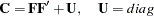For a first-order confirmatory factor analysis, you can use MATRIX statements to define elements in the matrices $\text{[math]}$ , $\text{[math]}$ , and $\text{[math]}$ of the more general model

$\text{[math]}$

To perform a component analysis, specify the COMPONENT option to constrain the matrix $\text{[math]}$ to a zero matrix; that is, the model is replaced by

$\text{[math]}$

Note that the rank of $\text{[math]}$ is equal to the number $\text{[math]}$ of components in $\text{[math]}$ , and if $\text{[math]}$ is smaller than the number of variables in the moment matrix $\text{[math]}$ , the matrix of predicted model values is singular and maximum likelihood estimates for $\text{[math]}$ cannot be computed. You should compute ULS estimates in this case.

The HEYWOOD option constrains the diagonal elements of $\text{[math]}$ to be nonnegative; that is, the model is replaced by

$\text{[math]}$

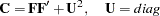If the factor loadings are unconstrained, they can be orthogonally rotated by one of the following methods:

principal axes rotation
quartimax
varimax
equamax
parsimax

The most common approach to factor analysis consists of two steps:

Obtain estimates for factor loadings and unique variances.
Apply an orthogonal or oblique rotation method.

PROC CALIS enables you to specify general linear and nonlinear equality and inequality constraints by using the LINCON and NLINCON statements. You can specify the NLINCON statement to estimate orthogonal or oblique rotated factor loadings; refer to Browne and Du Toit (1992). Unlike PROC FACTOR, PROC CALIS currently does not provide standard errors for the rotated factor loadings.

PROC CALIS also computes the factor score regression coefficients for the final factor solution.

For default (exploratory) factor analysis, PROC CALIS computes initial estimates. If you use a MATRIX statement together with a FACTOR model specification, initial values are generally computed by McDonald’s (McDonald and Hartmann 1992) method or are set by the START= option. See the section FACTOR Model Statement and Example 25.3 for more information about the FACTOR statement.

Constrained Estimation

Simple equality constraints $\text{[math]}$ and $\text{[math]}$ can be defined in each model by specifying constants or using the same name for parameters constrained to be equal.
BOUNDS statement: You can specify boundary constraints $\text{[math]}$ with the BOUNDS statement for the COSAN, LINEQS, and RAM models and in connection with an INRAM= data set. There might be serious convergence problems if negative values appear in the diagonal locations (variances) of the central model matrices during the minimization process. You can use the BOUNDS statement to constrain these parameters to have nonnegative values.
LINCON statement: You can specify general linear equality and inequality constraints of the parameter estimates with the LINCON statement or by using an INEST= data set. The variables listed in the LINCON statements must be (a subset of) the model parameters. All optimization methods can be used with linear constraints.
NLINCON statement: You can specify general nonlinear equality and inequality constraints of the parameter estimates with the NLINCON statement. The syntax of the NLINCON statement is almost the same as that for the BOUNDS statement with the exception that the BOUNDS statement can contain only names of the model parameters. However, the variables listed in the NLINCON statement can be defined by programming statements. Only the quasi-Newton optimization method can be used when there are nonlinear constraints.
Reparameterizing the model: Complex linear equality and inequality constraints can be defined by means of programming statements similar to those used in the DATA step. In this case, some of the parameters $\text{[math]}$ are not elements of the matrices $\text{[math]}$ and $\text{[math]}$ but are instead defined in a PARAMETERS statement. Elements of the model matrices can then be computed by programming statements as functions of parameters in the PARAMETERS statement. This approach is similar to the classical COSAN program of McDonald, implemented by Fraser (McDonald 1978, 1980). One advantage of the CALIS procedure is that you need not supply code for the derivatives of the specified functions. The analytic derivatives of the user-written functions are computed automatically by PROC CALIS. The specified functions must be continuous and have continuous first-order partial derivatives. See the section SAS Programming Statements and the section Constrained Estimation by Using Program Code for more information about imposing linear and nonlinear restrictions on parameters by using programming statements.

Although much effort has been made to implement reliable and numerically stable optimization methods, no practical algorithm exists that can always find the global optimum of a nonlinear function, especially when there are nonlinear constraints.

Top of Page