| The ACECLUS Procedure |
Getting Started: ACECLUS Procedure
The following example demonstrates how you can use the ACECLUS procedure to obtain approximate estimates of the pooled within-cluster covariance matrix and to compute canonical variables for subsequent analysis. You use PROC ACECLUS to preprocess data before you cluster it by using the FASTCLUS or CLUSTER procedure.
Suppose you want to determine whether national figures for birth rates, death rates, and infant death rates can be used to determine certain types or categories of countries. You want to perform a cluster analysis to determine whether the observations can be formed into groups suggested by the data. Previous studies indicate that the clusters computed from this type of data can be elongated and elliptical. Thus, you need to perform a linear transformation on the raw data before the cluster analysis.
The following data1 from Rouncefield (1995) are the birth rates, death rates, and infant death rates for 97 countries. The following statements create the SAS data set Poverty:
   data poverty;
      input Birth Death InfantDeath Country $15. @@;
      datalines;
   24.7  5.7  30.8 Albania         12.5 11.9  14.4 Bulgaria
   13.4 11.7  11.3 Czechoslovakia    12 12.4   7.6 Former_E._Germa
   11.6 13.4  14.8 Hungary         14.3 10.2    16 Poland
   13.6 10.7  26.9 Romania           14    9  20.2 Yugoslavia
   17.7   10    23 USSR            15.2  9.5  13.1 Byelorussia
   13.4 11.6    13 Ukrainian_SSR   20.7  8.4  25.7 Argentina
   46.6   18   111 Bolivia         28.6  7.9    63 Brazil
   23.4  5.8  17.1 Chile           27.4  6.1    40 Columbia
   32.9  7.4    63 Ecuador         28.3  7.3    56 Guyana
   34.8  6.6    42 Paraguay        32.9  8.3 109.9 Peru
   18    9.6  21.9 Uruguay         27.5  4.4  23.3 Venezuela
   29   23.2    43 Mexico            12 10.6   7.9 Belgium
   13.2 10.1   5.8 Finland         12.4 11.9   7.5 Denmark
   13.6  9.4   7.4 France          11.4 11.2   7.4 Germany
   10.1  9.2    11 Greece          15.1  9.1   7.5 Ireland
   9.7   9.1   8.8 Italy           13.2  8.6   7.1 Netherlands
   14.3 10.7   7.8 Norway          11.9  9.5  13.1 Portugal
   10.7  8.2   8.1 Spain           14.5 11.1   5.6 Sweden
   12.5  9.5   7.1 Switzerland     13.6 11.5   8.4 U.K.
   14.9  7.4     8 Austria          9.9  6.7   4.5 Japan
   14.5  7.3   7.2 Canada          16.7  8.1   9.1 U.S.A.
   40.4 18.7 181.6 Afghanistan     28.4  3.8    16 Bahrain
   42.5 11.5 108.1 Iran            42.6  7.8    69 Iraq
   22.3  6.3   9.7 Israel          38.9  6.4    44 Jordan
   26.8  2.2  15.6 Kuwait          31.7  8.7    48 Lebanon
   45.6  7.8    40 Oman            42.1  7.6    71 Saudi_Arabia
   29.2  8.4    76 Turkey          22.8  3.8    26 United_Arab_Emr
   42.2 15.5   119 Bangladesh      41.4 16.6   130 Cambodia
   21.2  6.7    32 China           11.7  4.9   6.1 Hong_Kong
   30.5 10.2    91 India           28.6  9.4    75 Indonesia
   23.5 18.1    25 Korea           31.6  5.6    24 Malaysia
   36.1  8.8    68 Mongolia        39.6 14.8   128 Nepal
   30.3  8.1 107.7 Pakistan        33.2  7.7    45 Philippines
   17.8  5.2   7.5 Singapore       21.3  6.2  19.4 Sri_Lanka
   22.3  7.7    28 Thailand        31.8  9.5    64 Vietnam
   35.5  8.3    74 Algeria         47.2 20.2   137 Angola
   48.5 11.6    67 Botswana        46.1 14.6    73 Congo
   38.8  9.5  49.4 Egypt           48.6 20.7   137 Ethiopia
   39.4 16.8   103 Gabon           47.4 21.4   143 Gambia
   44.4 13.1    90 Ghana             47 11.3    72 Kenya
   44    9.4    82  Libya          48.3   25   130 Malawi
   35.5  9.8    82 Morocco           45 18.5   141 Mozambique
   44   12.1   135 Namibia         48.5 15.6   105 Nigeria
   48.2 23.4   154 Sierra_Leone    50.1 20.2   132 Somalia
   32.1  9.9    72 South_Africa    44.6 15.8   108 Sudan
   46.8 12.5   118 Swaziland       31.1  7.3    52 Tunisia
   52.2 15.6   103 Uganda          50.5   14   106 Tanzania
   45.6 14.2    83 Zaire           51.1 13.7    80 Zambia
   41.7 10.3    66 Zimbabwe
   ;
The data set Poverty contains the character variable Country and the numeric variables Birth, Death, and InfantDeath, which represent the birth rate per thousand, death rate per thousand, and infant death rate per thousand, respectively. The $15. in the INPUT statement specifies that the variable Country is a character variable with a length of 15. The double trailing at sign (@@) in the INPUT statement specifies that observations are input from each line until all values have been read.
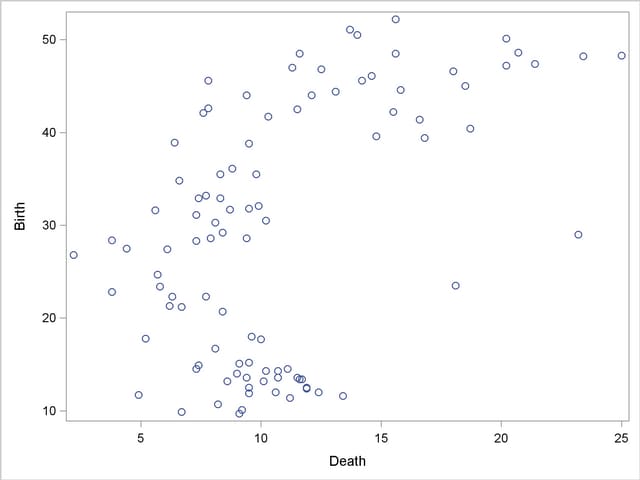
It is often useful when beginning a cluster analysis to look at the data graphically. The following statements use the SGPLOT procedure to make a scatter plot of the variables Birth and Death.
   proc sgplot data=poverty;
      scatter x=Death y=Birth;
   run;
The plot, displayed in Figure 22.1, indicates the difficulty of dividing the points into clusters. Plots of the other variable pairs (not shown) display similar characteristics. The clusters that comprise these data might be poorly separated and elongated. Data with poorly separated or elongated clusters must be transformed.
If you know the within-cluster covariances, you can transform the data to make the clusters spherical. However, since you do not know what the clusters are, you cannot calculate exactly the within-cluster covariance matrix. The ACECLUS procedure estimates the within-cluster covariance matrix to transform the data, even when you have no knowledge of cluster membership or the number of clusters.
The following statements perform the ACECLUS procedure transformation by using the SAS data set Poverty:
   proc aceclus data=poverty out=ace proportion=.03;
      var Birth Death InfantDeath;
   run;
The OUT= option creates an output data set called Ace to contain the canonical variable scores. The PROPORTION= option specifies that approximately 3 percent of the pairs are included in the estimation of the within-cluster covariance matrix. The VAR statement specifies that the variables Birth, Death, and InfantDeath are used in computing the canonical variables.
The results of this analysis are displayed in Figure 22.2 through Figure 22.5.
Figure 22.2 displays the number of observations, the number of variables, and the settings for the PROPORTION and CONVERGE options. The PROPORTION option is set at 0.03, as specified in the previous statements. The CONVERGE parameter is set at its default value of 0.001. Figure 22.2 next displays the means, standard deviations, and sample covariance matrix of the analytical variables.
| Observations | 97 | Proportion | 0.0300 |
|---|---|---|---|
| Variables | 3 | Converge | 0.00100 |
The type of matrix used for the initial within-cluster covariance estimate is displayed in Figure 22.3. In this example, that initial estimate is the full covariance matrix. The threshold value that corresponds to the PROPORTION=0.03 setting is given as 0.292815.
| Threshold = | 0.292815 |
|---|
| Iteration History | ||||
|---|---|---|---|---|
| Iteration | RMS Distance |
Distance Cutoff |
Pairs Within Cutoff |
Convergence Measure |
| 1 | 2.449 | 0.717 | 385.0 | 0.552025 |
| 2 | 12.534 | 3.670 | 446.0 | 0.008406 |
| 3 | 12.851 | 3.763 | 521.0 | 0.009655 |
| 4 | 12.882 | 3.772 | 591.0 | 0.011193 |
| 5 | 12.716 | 3.723 | 628.0 | 0.008784 |
| 6 | 12.821 | 3.754 | 658.0 | 0.005553 |
| 7 | 12.774 | 3.740 | 680.0 | 0.003010 |
| 8 | 12.631 | 3.699 | 683.0 | 0.000676 |
Figure 22.3 displays the iteration history. For each iteration, PROC ACECLUS displays the following measures:
root mean square distance between all pairs of observations
distance cutoff for including pairs of observations in the estimate of within-cluster covariances (equal to RMS*Threshold)
number of pairs within the cutoff
convergence measure
Figure 22.4 displays the approximate within-cluster covariance matrix and the table of eigenvalues from the canonical analysis. The first column of the eigenvalues table contains numbers for the eigenvectors. The next column of the table lists the eigenvalues of Inv(ACE)*(COV-ACE).
The next three columns of the eigenvalue table (Figure 22.4) display measures of the relative size and importance of the eigenvalues. The first column lists the difference between each eigenvalue and its successor. The last two columns display the individual and cumulative proportions that each eigenvalue contributes to the total sum of eigenvalues.
The raw and standardized canonical coefficients are displayed in Figure 22.5. The coefficients are standardized by multiplying the raw coefficients with the standard deviation of the associated variable. The ACECLUS procedure uses these standardized canonical coefficients to create the transformed canonical variables, which are the linear transformations of the original input variables, Birth, Death, and InfantDeath.
The following statements invoke the CLUSTER procedure, using the SAS data set Ace created in the previous ACECLUS procedure:
   proc cluster data=ace outtree=tree noprint method=ward;
      var can1 can2 can3 ;
      copy Birth--Country;
   run;
The OUTTREE= option creates the output SAS data set Tree that is used in subsequent statements to draw a tree diagram. The NOPRINT option suppresses the display of the output. The METHOD= option specifies Ward’s minimum-variance clustering method.
The VAR statement specifies that the canonical variables computed in the ACECLUS procedure are used in the cluster analysis. The COPY statement specifies that all the variables from the SAS data set Poverty (Birth—Country) are added to the output data set Tree.
The following statements use the TREE procedure to create an output SAS data set called New. The NCLUSTERS= option specifies the number of clusters desired in the SAS data set New. The NOPRINT option suppresses the display of the output.
   proc tree data=tree out=new nclusters=3 noprint;
      copy Birth Death InfantDeath can1 can2 ;
      id Country;
   run;
The COPY statement copies the canonical variables Can1 and Can2 (computed in the preceding ACECLUS procedure) and the original analytical variables Birth, Death, and InfantDeath into the output SAS data set New.
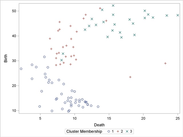
The following statements invoke the SGPLOT procedure, using the SAS data set created by PROC TREE:
   proc sgplot data=new;
      scatter y=Birth x= Death / group= cluster;
      keylegend / title= "Cluster Membership";
   run;
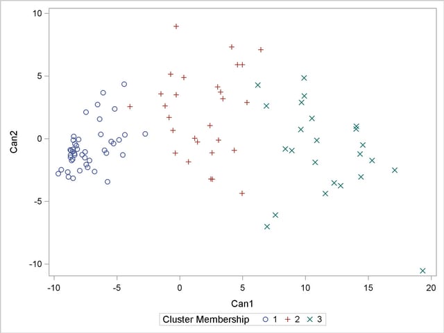
   proc sgplot data=new;
      scatter y=can2 x=can1 / group= cluster;
      keylegend / title= "Cluster Membership";
   run;
The first PROC SGPLOT statement requests a scatter plot of the two variables Birth and Death, using the variable CLUSTER as the identification variable.
The second PROC SGPLOT statement requests a plot of the two canonical variables, using the value of the variable CLUSTER as the identification variable.
Figure 22.6 and Figure 22.7 display the separation of the clusters when three clusters are calculated.
Copyright © 2009 by SAS Institute Inc., Cary, NC, USA. All rights reserved.