The HPSPLIT Procedure

Statistics that are printed in the subtree tables are similar to the pruning statistics. There are two ways to calculate the subtree statistics: one is based on a scored data set (using the SCORE statement or the SAS DATA step score code that the CODE statement produces), and the other is based on the internal observation counts at each leaf of the tree. The two methods should provide identical results unless the target is missing.
Note: The per-observation and per-leaf methods of calculating the subtree statistics might not agree if the input data set contains observations that have a missing value for the target.
In scoring, whether you use the SCORE
statement or you use the CODE
statement with a SAS DATA step, each observation is assigned a posterior probability, ![]() , where
, where ![]() is a target level. These posterior probabilities are then used to calculate the subtree statistics of the final tree.
is a target level. These posterior probabilities are then used to calculate the subtree statistics of the final tree.
For a leaf ![]() , the posterior probability is the fraction of observations at that leaf that have the target level
, the posterior probability is the fraction of observations at that leaf that have the target level ![]() . That is, for leaf
. That is, for leaf ![]() ,
,
When a record is scored, it is assigned to a leaf, and all posterior probabilities for that leaf are assigned along with
it. Thus, for observation ![]() assigned to leaf
assigned to leaf ![]() , the posterior probability is
, the posterior probability is
The variable ![]() continues to indicate the total number of observations in the input data set, and
continues to indicate the total number of observations in the input data set, and ![]() is the observation number (
is the observation number (![]() is used to prevent confusion with 0).
is used to prevent confusion with 0).
If a validation set is selected, the statistics are calculated separately for the validation set and for the training set.
In addition, the per-observation validation posterior probabilities should be used. The validation posterior probabilities,
![]() , are the same as the posterior probabilities from the training set, but they are the fraction of the observations from the
validation set that are in each target level,
, are the same as the posterior probabilities from the training set, but they are the fraction of the observations from the
validation set that are in each target level,
where ![]() and
and ![]() are now observation counts from the validation set. For calculating the statistics on the validation set, the same equations
can be used but substituting V for P where appropriate (for example,
are now observation counts from the validation set. For calculating the statistics on the validation set, the same equations
can be used but substituting V for P where appropriate (for example, ![]() for
for ![]() ).
).
The entropy at each observation is calculated from the posterior probabilities:
Like the entropy, the Gini statistic is also calculated from the posterior probabilities:
The misclassification rate is the average number of incorrectly predicted observations in the input data set. Predictions
are always based on the training set. Thus, each scored record’s predicted target level ![]() is compared against the actual level
is compared against the actual level ![]() :
:
![]() is the Kronecker delta:
is the Kronecker delta:
Phrased slightly differently, the misclassification rate is the fraction of incorrectly predicted observations:
For the sum of squares error (SSE), ![]() predictions are made for every observation: that the correct posterior is 1 and that the incorrect posteriors is 0. Thus
the SSE is as follows, where
predictions are made for every observation: that the correct posterior is 1 and that the incorrect posteriors is 0. Thus
the SSE is as follows, where ![]() is again the actual target level for observation
is again the actual target level for observation ![]() :
:
The subtree statistics that are calculated by PROC HPSPLIT are calculated per leaf. That is, instead of scanning through the entire data set, PROC HPSPLIT examines the proportions of observations at the leaves. Barring missing target values, which are not handled by the tree, the per-leaf and per-observation methods for calculating the subtree statistics are the same.
As with the per-observation method, observation counts N (![]() ,
, ![]() , and
, and ![]() ) can come from either the training set or the validation set. The growth subtree table always produces statistics from the
training set. The pruning subtree table produces both sets of data if they are both present.
) can come from either the training set or the validation set. The growth subtree table always produces statistics from the
training set. The pruning subtree table produces both sets of data if they are both present.
Unless otherwise marked, counts N can come from either set.
Because there are ![]() observations on the leaf
observations on the leaf ![]() , entropy takes the following form:
, entropy takes the following form:
Rephrased in terms of N, this becomes
The Gini statistic is similar to entropy in its leafwise form:
Rephrased in terms of N, this becomes
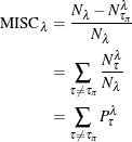
Misclassification comes from the number of incorrectly predicted observations. Thus, it is necessary to count the proportion of observations at each leaf in each target level. Similar to the misprediction rate of an entire data set, the misprediction rate of a single leaf, is
where the summation is over the observations that arrive at a leaf ![]() .
.
All observations at a leaf are assigned the same prediction because they are all assigned the same leaf. Therefore, the summation
reduces to simply the number of observations at leaf ![]() that have a target level other than the predicted target level for that leaf,
that have a target level other than the predicted target level for that leaf, ![]() . Thus,
. Thus,
where ![]() is
is ![]() if the validation set is being examined.
if the validation set is being examined.
Thus, for the entire data set, the misclassification rate is
where again ![]() is
is ![]() for the validation set.
for the validation set.
The sum of squares error (SSE) is treated similarly to the misclassification rate. Each observation is assigned per-target
posterior probabilities ![]() from the training data set. These are the predictions for the purpose of the SSE.
from the training data set. These are the predictions for the purpose of the SSE.
The observations at leaf ![]() are then grouped by the observations’ target levels. Because each observation in the group has the same actual target level,
are then grouped by the observations’ target levels. Because each observation in the group has the same actual target level,
![]() , and because all observations on the same node are assigned the same posterior probabilities,
, and because all observations on the same node are assigned the same posterior probabilities, ![]() , the per-observation SSE equation is identical:
, the per-observation SSE equation is identical:
![\begin{align*} \mathrm{SSE}_\Phi ^\lambda & = \sum _{\omega \in \Phi } \left[ \sum _{\tau \ne \tau _\pi ^\Phi } \left( P_{\tau }^\lambda \right)^2 + \left(1 - P_{\tau _\pi ^\Phi }^\lambda \right)^2 \right] \\ & = N_\Phi ^\lambda \left[ \sum _{\tau \ne \tau _\pi ^\Phi } \left( P_{\tau }^\lambda \right)^2 + \left(1 - P_{\tau _\pi ^\Phi }^\lambda \right)^2 \right] \end{align*}](images/stathpug_hpsplit0077.png)
Here, the posterior probabilities ![]() are from the training set, and the counts
are from the training set, and the counts ![]() are from whichever data set is being examined.
are from whichever data set is being examined.
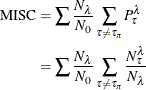
Thus, the SSE equation for the leaf can be rephrased in terms of a further summation over the target levels ![]() :
:
![\begin{equation*} \mathrm{SSE}_\lambda = \sum _\Phi N_\Phi ^\lambda \left[ \sum _{\tau \ne \tau _\pi ^\Phi } \left( P_{\tau }^\lambda \right)^2 + \left(1 - P_{\tau _\pi ^\Phi }^\lambda \right)^2 \right] \end{equation*}](images/stathpug_hpsplit0078.png)
So the SSE for the entire tree is then
![\begin{equation*} \mathrm{SSE} = \sum _\lambda \sum _\Phi N_\Phi ^\lambda \left[ \sum _{\tau \ne \tau _\pi ^\Phi } \left( P_{\tau }^\lambda \right)^2 + \left(1 - P_{\tau _\pi ^\Phi }^\lambda \right)^2 \right] \end{equation*}](images/stathpug_hpsplit0079.png)
Substituting the counts from the training set back in and using ![]() to denote training set counts, this becomes
to denote training set counts, this becomes
![\begin{align*} \mathrm{SSE} & = \sum _\lambda \sum _\Phi N_\Phi ^\lambda \left[ \sum _{\tau \ne \tau _\pi ^\Phi } \left( \frac{\nu _{\tau }^\lambda }{\nu _\lambda } \right)^2 + \left(1 - \frac{\nu _{\tau _\pi ^\Phi }^\lambda }{\nu _\lambda } \right)^2 \right] \\ & = \sum _\lambda \sum _\Phi N_\Phi ^\lambda \left[ \sum _{\tau \ne \tau _\pi ^\Phi } \left( \frac{\nu _{\tau }^\lambda }{\nu _\lambda } \right)^2 + 1 -2 \frac{\nu _{\tau _\pi ^\Phi }^\lambda }{\nu _\lambda } + \left( \frac{\nu _{\tau _\pi ^\Phi }^\lambda }{\nu _\lambda } \right)^2 \right] \\ & = \sum _\lambda \sum _\Phi N_\Phi ^\lambda \left[ \sum _{\tau } \left( \frac{\nu _{\tau }^\lambda }{\nu _\lambda } \right)^2 + 1 -2 \frac{\nu _{\tau _\pi ^\Phi }^\lambda }{\nu _\lambda } + \right] \\ & = \sum _\lambda N_\lambda \sum _\Phi \frac{N_\Phi ^\lambda }{N_\lambda } \left[ \sum _{\tau } \left( \frac{\nu _{\tau }^\lambda }{\nu _\lambda } \right)^2 + 1 -2 \frac{\nu _{\tau _\pi ^\Phi }^\lambda }{\nu _\lambda } \right] \\ & = \sum _\lambda N_\lambda \left[ 1 + \sum _{\tau } \left( \frac{\nu _{\tau }^\lambda }{\nu _\lambda } \right)^2 -2 \sum _\Phi \frac{N_\Phi ^\lambda }{N_\lambda } \frac{\nu _{\tau _\pi ^\Phi }^\lambda }{\nu _\lambda } \right] \end{align*}](images/stathpug_hpsplit0081.png)
In the rightmost inner summation, ![]() is simply
is simply ![]() , the target level being summed over. This gives the final equivalent forms
, the target level being summed over. This gives the final equivalent forms
![\begin{align*} \mathrm{SSE} & = \sum _\lambda N_\lambda \left[ 1 + \sum _{\tau } \left( \frac{\nu _{\tau }^\lambda }{\nu _\lambda } \right)^2 -2 \sum _\Phi \frac{N_\Phi ^\lambda }{N_\lambda } \frac{\nu _{\Phi }^\lambda }{\nu _\lambda } \right] \\ \mathrm{SSE} & = \sum _\lambda N_\lambda \left[ 1 + \sum _{\tau } \left( P_\tau ^\lambda \right)^2 -2 \sum _\Phi V_\Phi ^\lambda P_\Phi ^\lambda \right] \end{align*}](images/stathpug_hpsplit0083.png)
where ![]() and P are again counts and fraction, respectively, from the training set, and N and V are counts and fraction, respectively, from the validation set. (For example,
and P are again counts and fraction, respectively, from the training set, and N and V are counts and fraction, respectively, from the validation set. (For example, ![]() is the number of observations on leaf
is the number of observations on leaf ![]() that have target
that have target ![]() .)
.)
If there is no validation set, the training set is used instead, and the equations simplify to the following (because ![]() is merely an index over target levels and can be renamed
is merely an index over target levels and can be renamed ![]() ):
):
![\begin{align*} \mathrm{SSE} & = \sum _\lambda N_\lambda \left[ 1 - \sum _{\tau } \left( \frac{\nu _{\tau }^\lambda }{\nu _\lambda } \right)^2\right] \\ \mathrm{SSE} & = \sum _\lambda N_\lambda \left[ 1 - \sum _{\tau } \left( P_\tau ^\lambda \right)^2\right] \end{align*}](images/stathpug_hpsplit0085.png)
![\begin{align*} \mathrm{ASE} & = \sum _\lambda \frac{N_\lambda }{N_\tau N_0} \left[ 1 + \sum _{\tau } \left( \frac{\nu _{\tau }^\lambda }{\nu _\lambda } \right)^2 -2 \sum _\Phi \frac{N_\Phi ^\lambda }{N_\lambda } \frac{\nu _{\Phi }^\lambda }{\nu _\lambda } \right] \\ \mathrm{ASE} & = \sum _\lambda \frac{N_\lambda }{N_\tau N_0} \left[ 1 + \sum _{\tau } \left( P_\tau ^\lambda \right)^2 -2 \sum _\Phi V_\Phi ^\lambda P_\Phi ^\lambda \right] \end{align*}](images/stathpug_hpsplit0086.png)
![\begin{align*} \mathrm{SSE} & = \sum _\lambda \frac{N_\lambda }{N_\tau N_0} \left[ 1 - \sum _{\tau } \left( \frac{\nu _{\tau }^\lambda }{\nu _\lambda } \right)^2\right] \\ \mathrm{SSE} & = \sum _\lambda \frac{N_\lambda }{N_\tau N_0} \left[ 1 - \sum _{\tau } \left( P_\tau ^\lambda \right)^2\right] \end{align*}](images/stathpug_hpsplit0087.png)
Unlike a decision tree, regression trees model a continuous target. The predictions produced by a decision tree are based on the average of the partitioned space (the observations at the leaves).
As with decision trees, predictions come from the training set. The predicted value at leaf ![]() is
is
where the summation is over the observations i within leaf ![]() , and
, and ![]() is the value of the target variable at observation i within the training set.
is the value of the target variable at observation i within the training set.
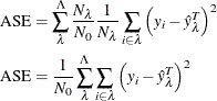
The observationwise sum of squares error (SSE) is the sum of squares of the difference between the observation’s value and
the value that is predicted for that observation, ![]() , which is equal to
, which is equal to ![]() where
where ![]() is the leaf to which that observation has been assigned, as described in the equation in the preceding section. The SSE is
then simply
is the leaf to which that observation has been assigned, as described in the equation in the preceding section. The SSE is
then simply
The leafwise sum of squares error (SSE) is related to the variance within that leaf. The training set SSE is identical to the sum of the variances within the leaves: