The HPLOGISTIC Procedure
-
Overview

-
Getting Started
-
Syntax
-
DetailsMissing ValuesResponse DistributionsLog-Likelihood FunctionsExistence of Maximum Likelihood EstimatesUsing Validation and Test DataModel Fit and Assessment StatisticsThe Hosmer-Lemeshow Goodness-of-Fit TestComputational Method: MultithreadingChoosing an Optimization AlgorithmDisplayed OutputODS Table Names
-
Examples
- References
The calculation of the information criteria uses the following formulas, where p denotes the number of effective parameters in the candidate model, F denotes the sum of frequencies used, and l is the log likelihood evaluated at the converged estimates:
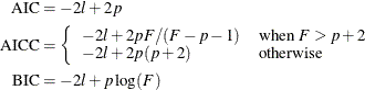
If you do not specify a FREQ statement, F equals n, the number of observations used.
The goal of a coefficient of determination, also known as an R-square measure, is to express the agreement between a stipulated model and the data in terms of variation in the data that is explained by the model. In linear models, the R-square measure is based on residual sums of squares; because these are additive, a measure bounded between 0 and 1 is easily derived.
In more general models where parameters are estimated by the maximum likelihood principle, Cox and Snell (1989, pp. 208–209) and Magee (1990) proposed the following generalization of the coefficient of determination:
Here, ![]() is the likelihood of the intercept-only model,
is the likelihood of the intercept-only model, ![]() is the likelihood of the specified model, and n denotes the number of observations used in the analysis. This number is adjusted for frequencies if a FREQ
statement is present and is based on the trials variable for binomial models.
is the likelihood of the specified model, and n denotes the number of observations used in the analysis. This number is adjusted for frequencies if a FREQ
statement is present and is based on the trials variable for binomial models.
As discussed in Nagelkerke (1991), this generalized R-square measure has properties similar to the coefficient of determination in linear models. If the model
effects do not contribute to the analysis, ![]() approaches
approaches ![]() and
and ![]() approaches zero.
approaches zero.
However, ![]() does not have an upper limit of 1. Nagelkerke suggested a rescaled generalized coefficient of determination,
does not have an upper limit of 1. Nagelkerke suggested a rescaled generalized coefficient of determination, ![]() , which achieves an upper limit of 1 by dividing
, which achieves an upper limit of 1 by dividing ![]() by its maximum value:
by its maximum value:
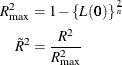
Another measure from McFadden (1974) is also bounded by 0 and 1:
If you specify the RSQUARE
option in the MODEL
statement, the HPLOGISTIC procedure computes ![]() and
and ![]() . All three measures are computed for each data role when you specify a PARTITION
statement.
. All three measures are computed for each data role when you specify a PARTITION
statement.
These measures are most useful for comparing competing models that are not necessarily nested—that is, models that cannot be reduced to one another by simple constraints on the parameter space. Larger values of the measures indicate better models.
For binary response data, the response Y is either an event or a nonevent; let the response Y take the value 1 for an event and 2 for a nonevent. From the fitted model, a predicted event probability ![]() can be computed for each observation i. If the predicted event probability equals or exceeds some cutpoint value
can be computed for each observation i. If the predicted event probability equals or exceeds some cutpoint value ![]() , the observation is classified as an event; otherwise, it is classified as a nonevent. Suppose
, the observation is classified as an event; otherwise, it is classified as a nonevent. Suppose ![]() of n individuals experience an event, such as a disease, and the remaining
of n individuals experience an event, such as a disease, and the remaining ![]() individuals are nonevents. The
individuals are nonevents. The ![]() decision matrix in Table 9.6 is obtained by cross-classifying the observed and predicted responses, where
decision matrix in Table 9.6 is obtained by cross-classifying the observed and predicted responses, where ![]() is the total number of observations that are observed to have Y=i and are classified into j. In this table, let
is the total number of observations that are observed to have Y=i and are classified into j. In this table, let ![]() denote an observed event and
denote an observed event and ![]() denote a nonevent, and let
denote a nonevent, and let ![]() indicate that the observation is classified as an event and
indicate that the observation is classified as an event and ![]() denote that the observation is classified as a nonevent.
denote that the observation is classified as a nonevent.
In the decision matrix, the number of true positives, ![]() , is the number of event observations that are correctly classified as events; the number of false positives,
, is the number of event observations that are correctly classified as events; the number of false positives, ![]() , is the number of nonevent observations that are incorrectly classified as events; the number of false negatives,
, is the number of nonevent observations that are incorrectly classified as events; the number of false negatives, ![]() , is the number of event observations that are incorrectly classified as nonevents; and the number of true negatives,
, is the number of event observations that are incorrectly classified as nonevents; and the number of true negatives, ![]() , is the number of nonevent observations that are correctly classified as nonevents. The following statistics are computed
from the preceding decision matrix:
, is the number of nonevent observations that are correctly classified as nonevents. The following statistics are computed
from the preceding decision matrix:
Table 9.7: Statistics from the Decision Matrix with Cutpoint z
|
Statistic |
Equation |
OUTROC Column |
|---|---|---|
|
Cutpoint |
z |
ProbLevel |
|
Number of true positives |
|
TruePos |
|
Number of true negatives |
|
TrueNeg |
|
Number of false positives |
|
FalsePos |
|
Number of false negatives |
|
FalseNeg |
|
Sensitivity |
|
TPF (true positive fraction) |
|
1–specificity |
|
FPF (false positive fraction) |
|
Correct classification rate |
|
PercentCorrect (PC) |
|
Misclassification rate |
1 – PC |
|
|
Positive predictive value |
|
PPV |
|
Negative predictive value |
|
NPV |
The accuracy of the classification is measured by its ability to predict events and nonevents correctly. Sensitivity (TPF, true positive fraction) is the proportion of event responses that are predicted to be events. Specificity (1–FPF, true negative fraction) is the proportion of nonevent responses that are predicted to be nonevents.
You can also measure accuracy by how well the classification predicts the response. The positive predictive value (PPV, 1–false positive rate) is the proportion of nonevents that are classified as events. The negative predictive value (NPV, 1–false negative rate) is the proportion of events that are classified as nonevents. The correct classification rate (PC) is the proportion of observations that are correctly classified.
If you also specify a PRIOR=
option, then PROC HPLOGISTIC uses Bayes’ theorem to modify the PPV, NPV, and PC as follows. Results of the classification
are represented by two conditional probabilities: sensitivity, ![]() , and one minus the specificity,
, and one minus the specificity, ![]() .
.
If the prevalence of the disease in the population ![]() is provided by the value of the PRIOR=
option, then the PPV, NPV, and PC are given by Fleiss (1981, pp. 4–5) as follows:
is provided by the value of the PRIOR=
option, then the PPV, NPV, and PC are given by Fleiss (1981, pp. 4–5) as follows:
![\begin{align*} \textnormal{PPV} & = {\Pr }(Y\! =\! 1|D\! =\! 1) = \frac{{\Pr }(Y\! =\! 1){\Pr }(D\! =\! 1|Y\! =\! 1)}{{\Pr }(D\! =\! 1|Y\! =\! 2) + {\Pr }(Y\! =\! 1)[{\Pr }(D\! =\! 1|Y\! =\! 1) - {\Pr }(D\! =\! 1|Y\! =\! 2)]} \\ \textnormal{NPV} & = {\Pr }(Y\! =\! 2|D\! =\! 2) = \frac{[1-{\Pr }(D\! =\! 1|Y\! =\! 2)]{[1-\Pr }(Y\! =\! 1)]}{1-{\Pr }(D\! =\! 1|Y\! =\! 2) - {\Pr }(Y\! =\! 1)[{\Pr }(D\! =\! 1|Y\! =\! 1) - {\Pr }(D\! =\! 1|Y\! =\! 2)]} \\ \textnormal{PC} & = {\Pr }(Y\! =\! 1|D\! =\! 1) + {\Pr }(Y\! =\! 2|D\! =\! 2) \\ & = {\Pr }(D\! =\! 1|Y\! =\! 1){\Pr }(Y\! =\! 1)+{\Pr }(D\! =\! 2|Y\! =\! 2)[1-{\Pr }(Y\! =\! 1)] \\ \end{align*}](images/stathpug_hplogistic0095.png)
If you do not specify the PRIOR= option, then PROC HPLOGISTIC uses the sample proportion of diseased individuals; that is,
![]() . In such a case, the preceding values reduce to those in Table 9.7. Note that for a stratified sampling situation in which
. In such a case, the preceding values reduce to those in Table 9.7. Note that for a stratified sampling situation in which ![]() and
and ![]() are chosen a priori,
are chosen a priori, ![]() is not a desirable estimate of
is not a desirable estimate of ![]() , so you should specify a PRIOR= option.
, so you should specify a PRIOR= option.
PROC HPLOGISTIC constructs the data for a receiver operating characteristic (ROC) curve by initially binning the predicted probabilities as discussed in the section The Hosmer-Lemeshow Goodness-of-Fit Test, then moving the cutpoint from 0 to 1 along the bin boundaries (so that the cutpoints correspond to the predicted probabilities), and then selecting those cutpoints where a change in the decision matrix occurs. The CTABLE option produces a table that includes these cutpoints and the statistics in Table 9.7 that correspond to each cutpoint. You can output this table to a SAS data set by specifying the CTABLE= option (see Table 9.7 for the column names), and you can display the ROC curve by using the SGPLOT procedure as shown in Example 9.2.
The area under the ROC curve (AUC), as determined by the trapezoidal rule, is given by the concordance index ![]() , which is described in the section Association Statistics.
, which is described in the section Association Statistics.
For more information about the topics in this section, see Pepe (2003).
The "Partition Fit Statistics" table displays the misclassification rate, true positive fraction, true negative fraction, and AUC according to their roles. If you have a polytomous response, then instead of classifying according to a cutpoint, PROC HPLOGISTIC classifies the observation into the lowest response level (which has the largest predicted probability for that observation) and similarly computes a true response-level fraction.
If you specify the ASSOCIATION option in the MODEL statement, PROC HPLOGISTIC displays measures of association between predicted probabilities and observed responses for binary or binomial response models. These measures assess the predictive ability of a model.
Of the n pairs of observations in the data set with different responses, let ![]() be the number of pairs where the observation that has the lower ordered response value has a lower predicted probability,
let
be the number of pairs where the observation that has the lower ordered response value has a lower predicted probability,
let ![]() be the number of pairs where the observation that has the lower ordered response value has a higher predicted probability,
and let
be the number of pairs where the observation that has the lower ordered response value has a higher predicted probability,
and let ![]() be the rest. Let N be the sum of observation frequencies in the data. Then the following statistics are reported:
be the rest. Let N be the sum of observation frequencies in the data. Then the following statistics are reported:
![\[ \begin{array}{lcl} \text {concordance index } C \text { (AUC)} & =& (n_ c+0.5n_ t)/n \\ \text {Somers’ } D \text { (Gini coefficient) } & =& (n_ c-n_ d)/n \\ \text {Goodman-Kruskal gamma } & =& (n_ c-n_ d)/(n_ c+n_ d) \\ \text {Kendall’s tau-}a & =& (n_ c-n_ d)/(0.5N(N-1)) \end{array} \]](images/stathpug_hplogistic0103.png)
Classification of the pairs is carried out by initially binning the predicted probabilities as discussed in the section The Hosmer-Lemeshow Goodness-of-Fit Test. The concordance index, C, is an estimate of the AUC, which is the area under the receiver operating characteristic (ROC) curve. If there are no ties, then Somers’ D (Gini’s coefficient) = 2C–1.
If you specify a PARTITION statement, then PROC HPLOGISTIC displays the AUC and Somers’ D in the "Association" and "Partition Fit Statistics" tables according to their roles.
The average squared error, ASE, is the average of the squared differences between the responses and the predictions. When you have a discrete number of response levels, the ASE is modified as shown in Table 9.8 (Brier, 1950; Murphy, 1973); it is also called the Brier score or Brier reliability:
Table 9.8: Average Square Error Computations
|
Response Type |
ASE (Brier Score) |
|---|---|
|
Polytomous |
|
|
Binary |
|
|
Binomial |
|
In Table 9.8, ![]() ,
, ![]() is the number of events,
is the number of events, ![]() is the number of trials in binomial response models, and
is the number of trials in binomial response models, and ![]() =1 for events and 0 for nonevents in binary response models. For polytomous response models,
=1 for events and 0 for nonevents in binary response models. For polytomous response models, ![]() =1 if the ith observation has response level j, and
=1 if the ith observation has response level j, and ![]() is the model-predicted probability of response level j for observation i.
is the model-predicted probability of response level j for observation i.
For a binary response model, write the mean of the model-predicted probabilities of event (Y=1) observations as ![]() and of the nonevent (Y=2) observations as
and of the nonevent (Y=2) observations as ![]() . The mean difference is
. The mean difference is ![]() , which Tjur (2009) relates to other R-square measures and calls the coefficient of discrimination because it is a measure of the model’s ability to distinguish between the event and nonevent distributions. This mean difference
is also the
, which Tjur (2009) relates to other R-square measures and calls the coefficient of discrimination because it is a measure of the model’s ability to distinguish between the event and nonevent distributions. This mean difference
is also the ![]() or
or ![]() statistic (with unit standard error) that is discussed in signal detection literature (McNicol, 2005).
statistic (with unit standard error) that is discussed in signal detection literature (McNicol, 2005).