Exploring Data in Three Dimensions

Rotating Plot with Fitted Surface

When you suspect that the values of one variable may be predicted by the values of two other variables, you can choose to fit a response surface to your data.

Follow these steps to explore how dust concentration varies with the wind speed and with the time of day in the AIR data set.

Open the AIR data set.

Choose Analyze:Rotating Plot ( Z Y X ).

[menu]
Figure 6.11: Creating a Rotating Plot with Fitted Surface

A rotating plot variables dialog appears, as shown in Figure 6.12.

Select DUST in the variables list at the left. Then click Z.

This assigns the Z role to the DUST variable. Similarly, assign HOUR the Y role and WIND the X role.

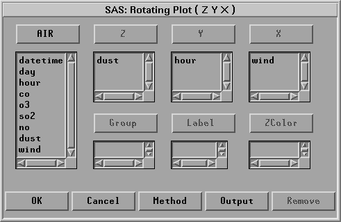
Figure 6.12: Rotating Plot Variables Dialog

Click Output to display the Output dialog, as shown in Figure 6.13.

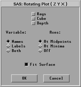
Figure 6.13: Output Dialog for Rotating Plot

Select Fit Surface and click OK.

Click Method to display the Method dialog, as shown in Figure 6.14.

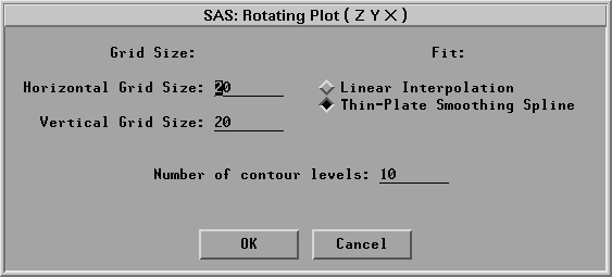
Figure 6.14: Method Dialog for Rotating Plot

Select Fit:Thin-Plate Smoothing Spline and click OK.

Click OK to create a surface plot.

Click on the menu button in the lower left corner of the plot.

Choose Drawing Modes:Smooth Color and Axes:At Minima.

Rotate the plot as described in the previous section.

You see a surface that models the response of dust concentration as a function of the wind speed and the time of day.

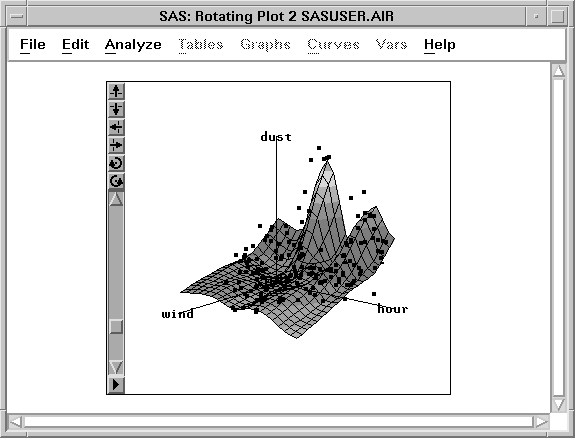
Figure 6.15: Rotating Plot with Fitted Surface

Top of Page