The MVPMONITOR Procedure

Example 13.1 Combining Data from Peer Processes
In some situations you might want to build a common principal component model by combining data from multiple peer processes that have similar patterns of stable variation. This enables you to borrow strength from the data. A common set of control limits is then computed for each peer process.
This example uses observations from all regions in the continental United States at each time value to construct a common principal component model. It then applies the model to flight data for one region.
The following statements create a principal component model that contains three principal components from the flightDelays data set and apply the model to data for the Midwest region:
proc mvpmodel data=flightDelays ncomp=3 noprint
              out=mvpair outloadings=mvpairloadings;
   var AA CO DL F9 FL NW UA US WN;
run;
proc mvpmonitor history=mvpair loadings=mvpairloadings;
   time flightDate;
   series region;
   spechart / seriesvalue='MW';
   tsquarechart / seriesvalue='MW';
run;
The flightDelays data set contains observations from all continental United States regions, with multiple observations (one for each region)
at each time point as defined by the flightDate variable. The OUTLOADINGS= data set that is produced by PROC MVPMODEL contains the model information. The SERIES statement specifies region as the variable that identifies sequences of related observations. The SERIESVALUE= option selects the Midwest region statistics to be plotted.
The resulting SPE chart is shown in Output 13.1.1.
Output 13.1.1: Multivariate Control Chart for SPE Statistics
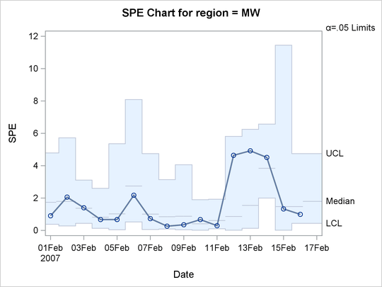
The control limits for the SPE chart are computed differently from a case with a single observation per time value, such as the chart shown in Figure 13.3. The control limits are based on different reference distributions for the SPE statistics in addition to different approximations to the reference distribution. See the section Computing SPE Control Limits for more information.
The ![]() chart is shown in Output 13.1.2.
chart is shown in Output 13.1.2.
Output 13.1.2: Multivariate Control Chart for ![]() Statistics
Statistics
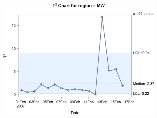
Compare the ![]() chart in Output 13.1.2 to the one in Figure 13.1. Both charts display
chart in Output 13.1.2 to the one in Figure 13.1. Both charts display ![]() statistics for the same flight delays from the Midwest region, but the charts are different because in this example the principal
component model was constructed with data from all regions of the continental United States.
statistics for the same flight delays from the Midwest region, but the charts are different because in this example the principal
component model was constructed with data from all regions of the continental United States.
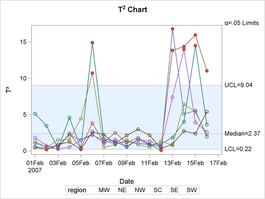
You can produce control charts for all the peer processes (regions in this example) by omitting the SERIESVALUE= option. The following statements illustrate this approach:
proc mvpmonitor history=mvpair;
   time flightDate;
   series region;
   spechart;
   tsquarechart / overlay;
run;
By default, a separate control chart is created for each distinct value of the SERIES variable. The separate SPE charts for
each region are not shown. The OVERLAY option in the TSQUARECHART statement specifies that the sequences for each region be plotted on a single ![]() chart, which is shown in Output 13.1.3.
chart, which is shown in Output 13.1.3.
Output 13.1.3: Overlaid ![]() Charts by Region
Charts by Region