| The SHEWHART Procedure |
Constructing Charts for Proportion Nonconforming (p Charts)
The following notation is used in this section:
|
expected proportion of nonconforming items produced by the process |
||||
|
proportion of nonconforming items in the |
||||
|
number of nonconforming items in the |
||||
|
number of items in the |
||||
|
average proportion of nonconforming items taken across subgroups:
|
||||
|
number of subgroups |
||||
|
incomplete beta function:
for |
 th subgroup
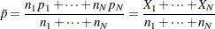


 ,
,  , and
, and  , where
  is the gamma function
 Plotted Points
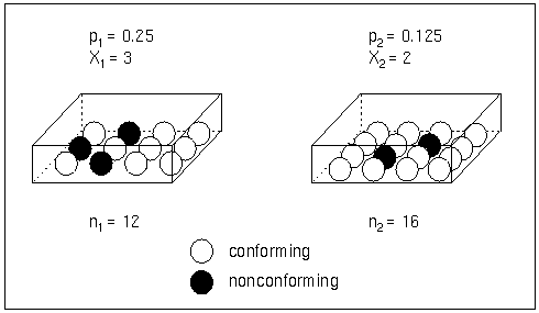
Each point on a  chart represents the observed proportion (
 ) of nonconforming items in a subgroup. For example, suppose the second subgroup (see Figure 13.21.12) contains 16 items, of which two are nonconforming. The point plotted for the second subgroup is
  .
.
Note that an  chart displays the number (count) of nonconforming items
  . You can use the NPCHART statement to create charts; see NPCHART Statement
Central Line
By default, the central line on a chart indicates an estimate of that is computed as  . If you specify a known value (
 ) for , the central line indicates the value of .
Control Limits
You can compute the limits in the following ways:
as a specified multiple (
 ) of the standard error of
  above and below the central line. The default limits are computed with
  (these are referred to as
  limits).
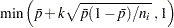
 as probability limits defined in terms of
 , a specified probability that
  exceeds the limits
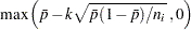
The lower and upper control limits, LCL and UCL, respectively, are computed as
 |
 |
 |
|||
 |
|
 |
A lower probability limit for can be determined using the fact that
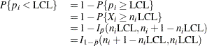 |
Refer to Johnson, Kotz, and Kemp (1992). This assumes that the process is in statistical control and that  is binomially distributed. The lower probability limit LCL is then calculated by setting
 |
and solving for LCL. Similarly, the upper probability limit for can be determined using the fact that
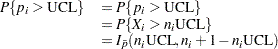 |
The upper probability limit UCL is then calculated by setting
 |
and solving for UCL. The probability limits are asymmetric around the central line. Note that both the control limits and probability limits vary with  .
.
You can specify parameters for the limits as follows:
Specify
with the SIGMAS= option or with the variable _SIGMAS_ in a LIMITS= data set. Specify
with the ALPHA= option or with the variable _ALPHA_ in a LIMITS= data set. Specify a constant nominal sample size
 for the control limits with the LIMITN= option or with the variable _LIMITN_ in a LIMITS= data set.
 Specify
with the P0= option or with the variable _P_ in a LIMITS= data set.
Copyright © SAS Institute, Inc. All Rights Reserved.