PROC RELIABILITY: Regression Model with Nonconstant Scale

The RELIABILITY Procedure

Regression Model with Nonconstant Scale

Nelson (1990, p. 272) and Meeker and Escobar (1998, p. 439) analyzed data from a strain-controlled fatigue test on 26 specimens of a type of superalloy. The following SAS statements create a SAS data set containing for each specimen the level of pseudo-stress (Pstress), the number of cycles (in thousands) (Kcycles) until failure or removal from the test, and a variable to indicate whether a specimen failed (F) or was right censored (C) (Status):

   data alloy;                           
      input pstress kcycles status$ @@;
      cen = ( status = 'C' );          
      datalines;                       
   80.3  211.629  F    99.8   43.331  F
   80.6  200.027  F   100.1   12.076  F
   80.8   57.923  C   100.5   13.181  F
   84.3  155.000  F   113.0   18.067  F
   85.2   13.949  F   114.8   21.300  F
   85.6  112.968  C   116.4   15.616  F
   85.8  152.680  F   118.0   13.030  F
   86.4  156.725  F   118.4    8.489  F
   86.7  138.114  C   118.6   12.434  F
   87.2   56.723  F   120.4    9.750  F
   87.3  121.075  F   142.5   11.865  F
   89.7  122.372  C   144.5    6.705  F
   91.3  112.002  F   145.9    5.733  F
   ;                                   
                                       
   run;

The following statements fit a Weibull regression model with the number of cycles to failure as the response variable:

ods output ModObstats = Resids;
proc reliability data = alloy;                                                 
   distribution weibull;                                                        
   model kcycles*cen(1) = pstress pstress*pstress / Relation = Pow Obstats;             
   logscale pstress;                                                            
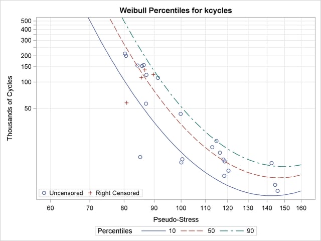
   rplot kcycles*cen(1) = pstress /  fit=regression                             
                                     relation = pow                             
                                     plotfit  10 50 90                          
                                     slower=60 supper=160                       
                                     lupper=500;                                
                                                                                
   label pstress = "Pseudo-Stress";                                             
   label kcycles = "Thousands of Cycles";                                       
run;

The data set RESIDS contains standardized residuals created with the ODS OUTPUT statement. The MODEL statement specifies a model quadratic in the log of pseudo-stress for the extreme value location parameter. The quadratic model in pseudo-stress PSTRESS is specified in the MODEL statement, and the RELATION=POW option specifies that the log transformation be applied to Pstress in the MODEL statement and the LOGSCALE statement. The LOGSCALE statement specifies the log of the scale parameter as a linear function of the log of Pstress. The RPLOT statement specifies a plot of the data and the fitted regression model versus the variable Pstress. The FIT=REGRESSION option specifies plotting the regression model fitted with the preceding MODEL statement. The RELATION=POW option specifies a log stress axis. The PLOTFIT option specifies plotting the 10th, 50th, and 90th percentiles of the regression model at each stress level. The SLOWER, SUPPER, and LUPPER options control limits on the stress and lifetime axes.

Figure 12.21 displays the parameter estimates from the fitted regression model. Parameter estimates for both the model for the location parameter and the scale parameter models are shown. Standard errors and confidence limits for all parameter estimates are included.

Figure 12.21 Parameter Estimates for Fitted Regression Model

The RELIABILITY Procedure

Weibull Parameter Estimates
Parameter	Estimate	Standard Error	Asymptotic Normal
			95% Confidence Limits
			Lower	Upper
Intercept	243.1681	58.0666	129.3596	356.9766
pstress	-96.5240	24.7075	-144.9498	-48.0983
pstress*pstress	9.6653	2.6247	4.5210	14.8095

Log-Scale Parameter Estimates
Parameter	Estimate	Standard Error	Asymptotic Normal
			95% Confidence Limits
			Lower	Upper
Intercept	4.4666	4.0724	-3.5152	12.4485
pstress	-1.1757	0.8731	-2.8870	0.5355

Figure 12.22 displays the plot of the data and fitted regression model.

Figure 12.22 Superalloy Fatigue Data with Fitted Regression Model

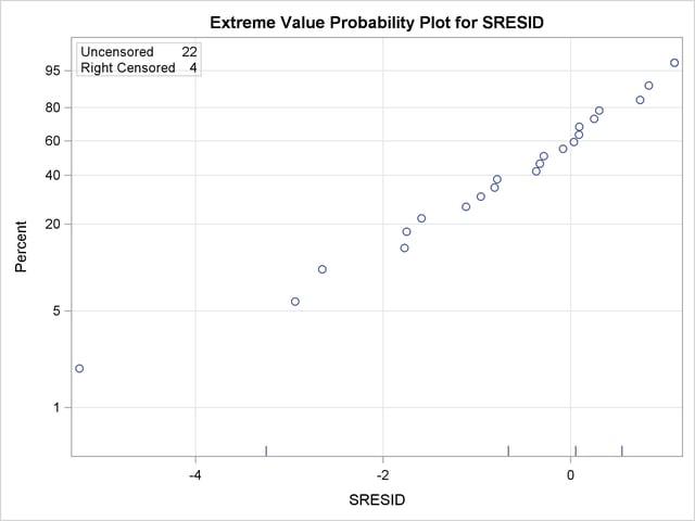
The following SAS statements create an extreme values probability plot of standardized residuals from the regression model shown in Figure 12.23:

proc reliability data = Resids;
   distribution ev;
   pplot sresid*cen(1) / nofit
                         ;
run;

Figure 12.23 Residuals for Superalloy Fatigue Data Regression Model

Top of Page