The UNIVARIATE Procedure
- Overview
-
Getting Started

-
Syntax
-
DetailsMissing ValuesRoundingDescriptive StatisticsCalculating the ModeCalculating PercentilesTests for LocationConfidence Limits for Parameters of the Normal DistributionRobust EstimatorsCreating Line Printer PlotsCreating High-Resolution GraphicsUsing the CLASS Statement to Create Comparative PlotsPositioning InsetsFormulas for Fitted Continuous DistributionsGoodness-of-Fit TestsKernel Density EstimatesConstruction of Quantile-Quantile and Probability PlotsInterpretation of Quantile-Quantile and Probability PlotsDistributions for Probability and Q-Q PlotsEstimating Shape Parameters Using Q-Q PlotsEstimating Location and Scale Parameters Using Q-Q PlotsEstimating Percentiles Using Q-Q PlotsInput Data SetsOUT= Output Data Set in the OUTPUT StatementOUTHISTOGRAM= Output Data SetOUTKERNEL= Output Data SetOUTTABLE= Output Data SetTables for Summary StatisticsODS Table NamesODS Tables for Fitted DistributionsODS GraphicsComputational Resources
-
ExamplesComputing Descriptive Statistics for Multiple VariablesCalculating ModesIdentifying Extreme Observations and Extreme ValuesCreating a Frequency TableCreating Plots for Line Printer OutputAnalyzing a Data Set With a FREQ VariableSaving Summary Statistics in an OUT= Output Data SetSaving Percentiles in an Output Data SetComputing Confidence Limits for the Mean, Standard Deviation, and VarianceComputing Confidence Limits for Quantiles and PercentilesComputing Robust EstimatesTesting for LocationPerforming a Sign Test Using Paired DataCreating a HistogramCreating a One-Way Comparative HistogramCreating a Two-Way Comparative HistogramAdding Insets with Descriptive StatisticsBinning a HistogramAdding a Normal Curve to a HistogramAdding Fitted Normal Curves to a Comparative HistogramFitting a Beta CurveFitting Lognormal, Weibull, and Gamma CurvesComputing Kernel Density EstimatesFitting a Three-Parameter Lognormal CurveAnnotating a Folded Normal CurveCreating Lognormal Probability PlotsCreating a Histogram to Display Lognormal FitCreating a Normal Quantile PlotAdding a Distribution Reference LineInterpreting a Normal Quantile PlotEstimating Three Parameters from Lognormal Quantile PlotsEstimating Percentiles from Lognormal Quantile PlotsEstimating Parameters from Lognormal Quantile PlotsComparing Weibull Quantile PlotsCreating a Cumulative Distribution PlotCreating a P-P Plot
- References
This example is a continuation of the example explored in the section Modeling a Data Distribution.
In the normal probability plot shown in Figure 4.6, the nonlinearity of the point pattern indicates a departure from normality in the distribution of Deviation. Because the point pattern is curved with slope increasing from left to right, a theoretical distribution that is skewed
to the right, such as a lognormal distribution, should provide a better fit than the normal distribution. See the section
Interpretation of Quantile-Quantile and Probability Plots.
You can explore the possibility of a lognormal fit with a lognormal probability plot. When you request such a plot, you must
specify the shape parameter ![]() for the lognormal distribution. This value must be positive, and typical values of
for the lognormal distribution. This value must be positive, and typical values of ![]() range from 0.1 to 1.0. You can specify values for
range from 0.1 to 1.0. You can specify values for ![]() with the SIGMA= secondary option in the LOGNORMAL primary option, or you can specify that
with the SIGMA= secondary option in the LOGNORMAL primary option, or you can specify that ![]() is to be estimated from the data.
is to be estimated from the data.
The following statements illustrate the first approach by creating a series of three lognormal probability plots for the variable
Deviation introduced in the section Modeling a Data Distribution:
symbol v=plus height=3.5pct;
title 'Lognormal Probability Plot for Position Deviations';
ods graphics off;
proc univariate data=Aircraft noprint;
   probplot Deviation /
      lognormal(theta=est zeta=est sigma=0.7 0.9 1.1)
      href  = 95
      lhref = 1
      square;
run;
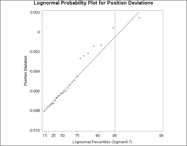
The LOGNORMAL primary option requests plots based on the lognormal family of distributions, and the SIGMA= secondary option
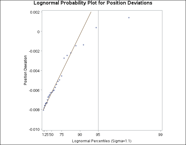
requests plots for ![]() equal to 0.7, 0.9, and 1.1. These plots are displayed in Output 4.26.1, Output 4.26.2, and Output 4.26.3, respectively. Alternatively, you can specify
equal to 0.7, 0.9, and 1.1. These plots are displayed in Output 4.26.1, Output 4.26.2, and Output 4.26.3, respectively. Alternatively, you can specify ![]() to be estimated using the sample standard deviation by using the option SIGMA=EST.
to be estimated using the sample standard deviation by using the option SIGMA=EST.
The SQUARE option displays the probability plot in a square format, the HREF= option requests a reference line at the 95th percentile, and the LHREF= option specifies the line type for the reference line.
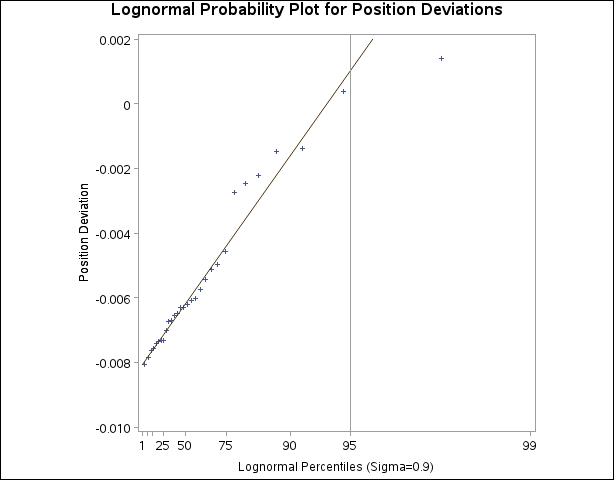
The value ![]() in Output 4.26.2 most nearly linearizes the point pattern. The 95th percentile of the position deviation distribution seen in Output 4.26.2 is approximately 0.001, because this is the value corresponding to the intersection of the point pattern with the reference
line.
in Output 4.26.2 most nearly linearizes the point pattern. The 95th percentile of the position deviation distribution seen in Output 4.26.2 is approximately 0.001, because this is the value corresponding to the intersection of the point pattern with the reference
line.
Note: After the ![]() that produces the most linear fit is found, you can then estimate the threshold parameter
that produces the most linear fit is found, you can then estimate the threshold parameter ![]() and the scale parameter
and the scale parameter ![]() . See Example 4.31.
. See Example 4.31.
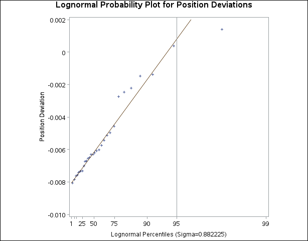
The following statements illustrate how you can create a lognormal probability plot for Deviation by using a local maximum likelihood estimate for ![]() .
.
symbol v=plus height=3.5pct;
title 'Lognormal Probability Plot for Position Deviations';
ods graphics off;
proc univariate data=Aircraft noprint;
   probplot Deviation / lognormal(theta=est zeta=est sigma=est)
                        href   = 95
                        square;
run;
The plot is displayed in Output 4.26.4. Note that the maximum likelihood estimate of ![]() (in this case, 0.882) does not necessarily produce the most linear point pattern.
(in this case, 0.882) does not necessarily produce the most linear point pattern.
A sample program for this example, uniex16.sas, is available in the SAS Sample Library for Base SAS software.