Alternatives for Producing Graphics

The UNIVARIATE procedure supports two kinds of graphical output:

• traditional graphics

• ODS Statistical Graphics output

PROC UNIVARIATE produces traditional graphics by default. These graphs are saved in graphics catalogs. Their appearance is controlled by the SAS/GRAPH GOPTIONS, AXIS, and SYMBOL statements (as described in SAS/GRAPH: Reference) and numerous specialized plot statement options.

ODS Statistical Graphics (or ODS Graphics for short) is an extension to the Output Delivery System (ODS) that is invoked when you use the ODS GRAPHICS statement prior to your procedure statements. An ODS graph is produced in ODS output (not a graphics catalog), and the details of its appearance and layout are controlled by ODS styles and templates rather than by SAS/GRAPH statements and procedure options. See Chapter 21, Statistical Graphics Using ODS (SAS/STAT 9.22 User's Guide), for a thorough discussion of ODS Graphics.

Prior to SAS 9.2, the plots produced by PROC UNIVARIATE were extremely basic by default. Producing attractive graphical output required the careful selection of colors, fonts, and other elements, which were specified via SAS/GRAPH statements and plot statement options. Beginning with SAS 9.2, the default appearance of traditional graphs is governed by the prevailing ODS style, which automatically produces attractive, consistent output. The SAS/GRAPH statements and procedure options for controlling graph appearance continue to be honored for traditional graphics. You can specify the NOGSTYLE system option to prevent the ODS style from affecting the appearance of traditional graphs. This enables existing PROC UNIVARIATE programs to produce customized graphs that appear as they did under previous SAS releases.

The appearance of ODS Graphics output is also controlled by the ODS style, but it is not affected by SAS/GRAPH statements or plot statement options that govern traditional graphics, For example, the CAXIS= option used to specify the color of graph axes in traditional graphics is ignored when producing ODS Graphics output. Note:Some features available with traditional graphics are not supported in ODS Graphics by the UNIVARIATE procedure for SAS 9.2.

The traditional graphics system enables you to control every detail of a graph through convenient procedure syntax. ODS Graphics provides the highest quality output with minimal syntax and full compatibility with graphics produced by SAS/STAT and SAS/ETS procedures.

The following code produces a histogram with a fitted lognormal distribution of the LoanToValueRatio data introduced in the section Summarizing a Data Distribution:

options nogstyle;
proc univariate data=HomeLoans noprint;
   histogram LoanToValueRatio / lognormal;
   inset lognormal(theta sigma zeta) / position=ne;
run;

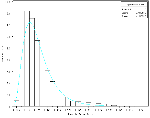
The NOGSTYLE system option keeps the ODS style from influencing the output, and no SAS/GRAPH statements or procedure options affecting the appearance of the plot are specified. Figure 4.8 shows the resulting histogram, which is essentially identical to the default output produced under releases prior to SAS 9.2.

Figure 4.8 Traditional Graph with NOGSTYLE

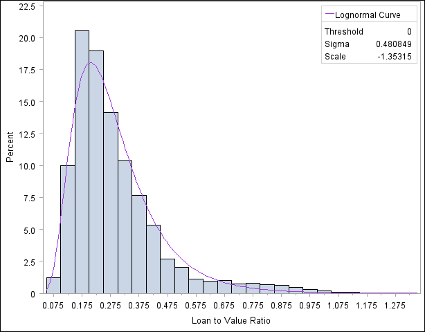
Figure 4.9 shows the result of executing the same code with the GSTYLE system option turned on (the default). Note the influence of the ODS style on the histogram’s appearance. For example, the quality of the text is improved and histogram bars are filled by default.

Figure 4.9 Traditional Graph with GSTYLE

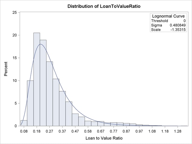
Figure 4.10 shows the same histogram produced using ODS Graphics. The histogram’s appearance is governed by the same style elements as in Figure 4.9, but the plots are not identical. Note, for example, the title incorporated in the ODS Graphics output and the smoother appearance of the fitted curve.

Figure 4.10 ODS Graphics Output