PROC UNIVARIATE: HISTOGRAM Statement

The UNIVARIATE Procedure

HISTOGRAM Statement

HISTOGRAM <variables> < / options> ;

The HISTOGRAM statement creates histograms and optionally superimposes estimated parametric and nonparametric probability density curves. You cannot use the WEIGHT statement with the HISTOGRAM statement. You can use any number of HISTOGRAM statements after a PROC UNIVARIATE statement. The components of the HISTOGRAM statement are follows.

variables

are the variables for which histograms are to be created. If you specify a VAR statement, the variables must also be listed in the VAR statement. Otherwise, the variables can be any numeric variables in the input data set. If you do not specify variables in a VAR statement or in the HISTOGRAM statement, then by default, a histogram is created for each numeric variable in the DATA= data set. If you use a VAR statement and do not specify any variables in the HISTOGRAM statement, then by default, a histogram is created for each variable listed in the VAR statement.

For example, suppose a data set named Steel contains exactly two numeric variables named Length and Width. The following statements create two histograms, one for Length and one for Width:

   proc univariate data=Steel;
      histogram;
   run;

Likewise, the following statements create histograms for Length and Width:

   proc univariate data=Steel;
      var Length Width;
      histogram;
   run;

The following statements create a histogram for Length only:

   proc univariate data=Steel;
      var Length Width;
      histogram Length;
   run;

options

add features to the histogram. Specify all options after the slash (/) in the HISTOGRAM statement. Options can be one of the following:

primary options for fitted parametric distributions and kernel density estimates
secondary options for fitted parametric distributions and kernel density estimates
general options for graphics and output data sets

For example, in the following statements, the NORMAL option displays a fitted normal curve on the histogram, the MIDPOINTS= option specifies midpoints for the histogram, and the CTEXT= option specifies the color of the text:

   proc univariate data=Steel;
      histogram Length / normal
                         midpoints = 5.6 5.8 6.0 6.2 6.4
                         ctext     = blue;
   run;

Table 4.11 through Table 4.23 list the HISTOGRAM options by function. For complete descriptions, see the sections Dictionary of Options and Dictionary of Common Options.

Parametric Density Estimation Options

Table 4.11 lists primary options that display parametric density estimates on the histogram. You can specify each primary option once in a given HISTOGRAM statement, and each primary option can display multiple curves from its family on the histogram.

Table 4.11 Primary Options for Parametric Fitted Distributions
Option	Description
BETA(beta-options)	fits beta distribution with threshold parameter $\text{[math]}$ , scale parameter $\text{[math]}$ , and shape parameters $\text{[math]}$ and $\text{[math]}$
EXPONENTIAL(exponential-options)	fits exponential distribution with threshold parameter $\text{[math]}$ and scale parameter $\text{[math]}$
GAMMA(gamma-options)	fits gamma distribution with threshold parameter $\text{[math]}$ , scale parameter $\text{[math]}$ , and shape parameter $\text{[math]}$
LOGNORMAL(lognormal-options)	fits lognormal distribution with threshold parameter $\text{[math]}$ , scale parameter $\text{[math]}$ , and shape parameter $\text{[math]}$
NORMAL(normal-options)	fits normal distribution with mean $\text{[math]}$ and standard deviation $\text{[math]}$
SB( $\text{[math]}$ -options)	fits Johnson $\text{[math]}$ distribution with threshold parameter $\text{[math]}$ , scale parameter $\text{[math]}$ , and shape parameters $\text{[math]}$ and $\text{[math]}$
SU( $\text{[math]}$ -options)	fits Johnson $\text{[math]}$ distribution with threshold parameter $\text{[math]}$ , scale parameter $\text{[math]}$ , and shape parameters $\text{[math]}$ and $\text{[math]}$
WEIBULL(Weibull-options)	fits Weibull distribution with threshold parameter $\text{[math]}$ , scale parameter $\text{[math]}$ , and shape parameter $\text{[math]}$

Table 4.12 through Table 4.20 list secondary options that specify parameters for fitted parametric distributions and that control the display of fitted curves. Specify these secondary options in parentheses after the primary distribution option. For example, you can fit a normal curve by specifying the NORMAL option as follows:

   proc univariate;
      histogram / normal(color=red mu=10 sigma=0.5);
   run;

The COLOR= normal-option draws the curve in red, and the MU= and SIGMA= normal-options specify the parameters $\text{[math]}$ and $\text{[math]}$ for the curve. Note that the sample mean and sample standard deviation are used to estimate $\text{[math]}$ and $\text{[math]}$ , respectively, when the MU= and SIGMA= normal-options are not specified.

You can specify lists of values for secondary options to display more than one fitted curve from the same distribution family on a histogram. Option values are matched by list position. You can specify the value EST in a list of distribution parameter values to use an estimate of the parameter.

For example, the following code displays two normal curves on a histogram:

   proc univariate;
      histogram / normal(color=(red blue) mu=10 est sigma=0.5 est);
   run;

The first curve is red, with $\text{[math]}$ and $\text{[math]}$ . The second curve is blue, with $\text{[math]}$ equal to the sample mean and $\text{[math]}$ equal to the sample standard deviation.

See the section Formulas for Fitted Continuous Distributions for detailed information about the families of parametric distributions that you can fit with the HISTOGRAM statement.

Table 4.12 Secondary Options Used with All Parametric Distribution Options
Option	Description
COLOR=	specifies colors of density curves
CONTENTS=	specifies table of contents entry for density curve grouping
FILL	fills area under density curve
L=	specifies line types of density curves
MIDPERCENTS	prints table of midpoints of histogram intervals
NOPRINT	suppresses tables summarizing curves
PERCENTS=	lists percents for which quantiles calculated from data and quantiles estimated from curves are tabulated
W=	specifies widths of density curves

Table 4.13 Secondary Beta-Options
Option	Description
ALPHA=	specifies first shape parameter $\text{[math]}$ for beta curve
BETA=	specifies second shape parameter $\text{[math]}$ for beta curve
SIGMA=	specifies scale parameter $\text{[math]}$ for beta curve
THETA=	specifies lower threshold parameter $\text{[math]}$ for beta curve

Table 4.14 Secondary Exponential-Options
Option	Description
SIGMA=	specifies scale parameter $\text{[math]}$ for exponential curve
THETA=	specifies threshold parameter $\text{[math]}$ for exponential curve

Table 4.15 Secondary Gamma-Options
Option	Description
ALPHA=	specifies shape parameter $\text{[math]}$ for gamma curve
ALPHADELTA=	specifies change in successive estimates of $\text{[math]}$ at which the Newton-Raphson approximation of $\text{[math]}$ terminates
ALPHAINITIAL=	specifies initial value for $\text{[math]}$ in the Newton-Raphson approximation of $\text{[math]}$
MAXITER=	specifies maximum number of iterations in the Newton-Raphson approximation of $\text{[math]}$
SIGMA=	specifies scale parameter $\text{[math]}$ for gamma curve
THETA=	specifies threshold parameter $\text{[math]}$ for gamma curve

Table 4.16 Secondary Lognormal-Options
Option	Description
SIGMA=	specifies shape parameter $\text{[math]}$ for lognormal curve
THETA=	specifies threshold parameter $\text{[math]}$ for lognormal curve
ZETA=	specifies scale parameter $\text{[math]}$ for lognormal curve

Table 4.17 Secondary Normal-Options
Option	Description
MU=	specifies mean $\text{[math]}$ for normal curve
SIGMA=	specifies standard deviation $\text{[math]}$ for normal curve

Table 4.18 Secondary Johnson $\text{[math]}$ -Options
Option	Description
DELTA=	specifies first shape parameter $\text{[math]}$ for Johnson $\text{[math]}$ curve
FITINTERVAL=	specifies $\text{[math]}$ -value for method of percentiles
FITMETHOD=	specifies method of parameter estimation
FITTOLERANCE=	specifies tolerance for method of percentiles
GAMMA=	specifies second shape parameter $\text{[math]}$ for Johnson $\text{[math]}$ curve
SIGMA=	specifies scale parameter $\text{[math]}$ for Johnson $\text{[math]}$ curve
THETA=	specifies lower threshold parameter $\text{[math]}$ for Johnson $\text{[math]}$ curve

Table 4.19 Secondary Johnson $\text{[math]}$ -Options
Option	Description
DELTA=	specifies first shape parameter $\text{[math]}$ for Johnson $\text{[math]}$ curve
FITINTERVAL=	specifies $\text{[math]}$ -value for method of percentiles
FITMETHOD=	specifies method of parameter estimation
FITTOLERANCE=	specifies tolerance for method of percentiles
GAMMA=	specifies second shape parameter $\text{[math]}$ for Johnson $\text{[math]}$ curve
SIGMA=	specifies scale parameter $\text{[math]}$ for Johnson $\text{[math]}$ curve
THETA=	specifies lower threshold parameter $\text{[math]}$ for Johnson $\text{[math]}$ curve

Table 4.20 Secondary Weibull-Options
Option	Description
C=	specifies shape parameter c for Weibull curve
CDELTA=	specifies change in successive estimates of $\text{[math]}$ at which the Newton-Raphson approximation of $\text{[math]}$ terminates
CINITIAL=	specifies initial value for $\text{[math]}$ in the Newton-Raphson approximation of $\text{[math]}$
MAXITER=	specifies maximum number of iterations in the Newton-Raphson approximation of $\text{[math]}$
SIGMA=	specifies scale parameter $\text{[math]}$ for Weibull curve
THETA=	specifies threshold parameter $\text{[math]}$ for Weibull curve

Nonparametric Density Estimation Options

Use the option KERNEL(kernel-options) to compute kernel density estimates. Specify the following secondary options in parentheses after the KERNEL option to control features of density estimates requested with the KERNEL option.

Table 4.21 Kernel-Options
Option	Description
C=	specifies standardized bandwidth parameter $\text{[math]}$
COLOR=	specifies color of the kernel density curve
FILL	fills area under kernel density curve
K=	specifies type of kernel function
L=	specifies line type used for kernel density curve
LOWER=	specifies lower bound for kernel density curve
UPPER=	specifies upper bound for kernel density curve
W=	specifies line width for kernel density curve

General Options

Table 4.22 summarizes options for enhancing histograms, and Table 4.23 summarizes options for requesting output data sets.

Table 4.22 General Graphics Options
Option	Description
ANNOKEY	applies annotation requested in ANNOTATE= data set to key cell only
ANNOTATE=	specifies annotate data set
BARLABEL=	produces labels above histogram bars
BARWIDTH=	specifies width for the bars
CAXIS=	specifies color for axis
CBARLINE=	specifies color for outlines of histogram bars
CFILL=	specifies color for filling under curve
CFRAME=	specifies color for frame
CFRAMESIDE=	specifies color for filling frame for row labels
CFRAMETOP=	specifies color for filling frame for column labels
CGRID=	specifies color for grid lines
CHREF=	specifies color for HREF= lines
CLIPREF	draws reference lines behind histogram bars
CONTENTS=	specifies table of contents entry for histogram grouping
CPROP=	specifies color for proportion of frequency bar
CTEXT=	specifies color for text
CTEXTSIDE=	specifies color for row labels of comparative histograms
CTEXTTOP=	specifies color for column labels of comparative histograms
CVREF=	specifies color for VREF= lines
DESCRIPTION=	specifies description for plot in graphics catalog
ENDPOINTS=	lists endpoints for histogram intervals
FONT=	specifies software font for text
FORCEHIST	forces creation of histogram
FRONTREF	draws reference lines in front of histogram bars
GRID	creates a grid
HANGING	constructs hanging histogram
HAXIS=	specifies AXIS statement for horizontal axis
HEIGHT=	specifies height of text used outside framed areas
HMINOR=	specifies number of horizontal minor tick marks
HOFFSET=	specifies offset for horizontal axis
HREF=	specifies reference lines perpendicular to the horizontal axis
HREFLABELS=	specifies labels for HREF= lines
HREFLABPOS=	specifies vertical position of labels for HREF= lines
INFONT=	specifies software font for text inside framed areas
INHEIGHT=	specifies height of text inside framed areas
INTERBAR=	specifies space between histogram bars
INTERTILE=	specifies distance between tiles
LGRID=	specifies a line type for grid lines
LHREF=	specifies line style for HREF= lines
LVREF=	specifies line style for VREF= lines
MAXNBIN=	specifies maximum number of bins to display
MAXSIGMAS=	limits the number of bins that display to within a specified number of standard deviations above and below mean of data in key cell
MIDPOINTS=	specifies midpoints for histogram intervals
NAME=	specifies name for plot in graphics catalog
NCOLS=	specifies number of columns in comparative histogram
NENDPOINTS=	specifies number of histogram interval endpoints
NMIDPOINTS=	specifies number of histogram interval midpoints
NOBARS	suppresses histogram bars
NOFRAME	suppresses frame around plotting area
NOHLABEL	suppresses label for horizontal axis
NOPLOT	suppresses plot
NOTABCONTENTS	suppresses table of contents entries for tables produced by HISTOGRAM statement
NOVLABEL	suppresses label for vertical axis
NOVTICK	suppresses tick marks and tick mark labels for vertical axis
NROWS=	specifies number of rows in comparative histogram
PFILL=	specifies pattern for filling under curve
RTINCLUDE	includes right endpoint in interval
TURNVLABELS	turns and vertically strings out characters in labels for vertical axis
VAXIS=	specifies AXIS statement or values for vertical axis
VAXISLABEL=	specifies label for vertical axis
VMINOR=	specifies number of vertical minor tick marks
VOFFSET=	specifies length of offset at upper end of vertical axis
VREF=	specifies reference lines perpendicular to the vertical axis
VREFLABELS=	specifies labels for VREF= lines
VREFLABPOS=	specifies horizontal position of labels for VREF= lines
VSCALE=	specifies scale for vertical axis
WAXIS=	specifies line thickness for axes and frame
WBARLINE=	specifies line thickness for bar outlines
WGRID=	specifies line thickness for grid

Table 4.23 Options for Requesting Output Data Sets
Option	Description
MIDPERCENTS	creates table of histogram intervals
OUTHISTOGRAM=	specifies information about histogram intervals
OUTKERNEL=	creates a data set containing kernel density estimates

Dictionary of Options

The following entries provide detailed descriptions of options in the HISTOGRAM statement. See the section Dictionary of Common Options for detailed descriptions of options common to all plot statements.

ALPHA=value-list

specifies the shape parameter $\text{[math]}$ for fitted curves requested with the BETA and GAMMA options. Enclose the ALPHA= option in parentheses after the BETA or GAMMA options. By default, or if you specify the value EST, the procedure calculates a maximum likelihood estimate for $\text{[math]}$ . You can specify A= as an alias for ALPHA= if you use it as a beta-option. You can specify SHAPE= as an alias for ALPHA= if you use it as a gamma-option.

BARLABEL=COUNT | PERCENT | PROPORTION

displays labels above the histogram bars. If you specify BARLABEL=COUNT, the label shows the number of observations associated with a given bar. If you specify BARLABEL=PERCENT, the label shows the percentage of observations represented by that bar. If you specify BARLABEL=PROPORTION, the label displays the proportion of observations associated with the bar.

BARWIDTH=value

specifies the width of the histogram bars in percentage screen units. If both the BARWIDTH= and INTERBAR= options are specified, the INTERBAR= option takes precedence.

BETA <(beta-options)>

displays fitted beta density curves on the histogram. The BETA option can occur only once in a HISTOGRAM statement, but it can request any number of beta curves. The beta distribution is bounded below by the parameter $\text{[math]}$ and above by the value $\text{[math]}$ . Use the THETA= and SIGMA= beta-options to specify these parameters. By default, THETA=0 and SIGMA=1. You can specify THETA=EST and SIGMA=EST to request maximum likelihood estimates for $\text{[math]}$ and $\text{[math]}$ .

The beta distribution has two shape parameters: $\text{[math]}$ and $\text{[math]}$ . If these parameters are known, you can specify their values with the ALPHA= and BETA= beta-options. By default, the procedure computes maximum likelihood estimates for $\text{[math]}$ and $\text{[math]}$ . Note:Three- and four-parameter maximum likelihood estimation may not always converge.

Table 4.12 and Table 4.13 list secondary options you can specify with the BETA option. See the section Beta Distribution for details and Example 4.21 for an example that uses the BETA option.

BETA=value-list

B=value-list

specifies the second shape parameter $\text{[math]}$ for beta density curves requested with the BETA option. Enclose the BETA= option in parentheses after the BETA option. By default, or if you specify the value EST, the procedure calculates a maximum likelihood estimate for $\text{[math]}$ .

C=value-list

specifies the shape parameter $\text{[math]}$ for Weibull density curves requested with the WEIBULL option. Enclose the C= Weibull-option in parentheses after the WEIBULL option. By default, or if you specify the value EST, the procedure calculates a maximum likelihood estimate for $\text{[math]}$ . You can specify the SHAPE= Weibull-option as an alias for the C= Weibull-option.

C=value-list

specifies the standardized bandwidth parameter $\text{[math]}$ for kernel density estimates requested with the KERNEL option. Enclose the C= kernel-option in parentheses after the KERNEL option. You can specify a list of values to request multiple estimates. You can specify the value MISE to produce the estimate with a bandwidth that minimizes the approximate mean integrated square error (MISE), or SJPI to select the bandwidth by using the Sheather-Jones plug-in method.

You can also use the C= kernel-option with the K= kernel-option (which specifies the kernel function) to compute multiple estimates. If you specify more kernel functions than bandwidths, the last bandwidth in the list is repeated for the remaining estimates. Similarly, if you specify more bandwidths than kernel functions, the last kernel function is repeated for the remaining estimates. If you do not specify the C= kernel-option, the bandwidth that minimizes the approximate MISE is used for all the estimates.

See the section Kernel Density Estimates for more information about kernel density estimates.

CBARLINE=color

specifies the color for the outline of the histogram bars when producing traditional graphics. The option does not apply to ODS Graphics output.

CFILL=color

specifies the color to fill the bars of the histogram (or the area under a fitted density curve if you also specify the FILL option) when producing traditional graphics. See the entries for the FILL and PFILL= options for additional details. Refer to SAS/GRAPH: Reference for a list of colors. The option does not apply to ODS Graphics output.

CGRID=color

specifies the color for grid lines when a grid displays on the histogram in traditional graphics. This option also produces a grid if the GRID= option is not specified.

CLIPREF

draws reference lines requested with the HREF= and VREF= options behind the histogram bars. When the GSTYLE system option is in effect for traditional graphics, reference lines are drawn in front of the bars by default.

CONTENTS=

specifies the table of contents grouping entry for tables associated with a density curve. Enclose the CONTENTS= option in parentheses after the distribution option. You can specify CONTENTS='' to suppress the grouping entry.

DELTA=value-list

specifies the first shape parameter $\text{[math]}$ for Johnson $\text{[math]}$ and Johnson $\text{[math]}$ distribution functions requested with the SB and SU options. Enclose the DELTA= option in parentheses after the SB or SU option. If you do not specify a value for $\text{[math]}$ , or if you specify the value EST, the procedure calculates an estimate.

ENDPOINTS <=values | KEY | UNIFORM>

uses histogram bin endpoints as the tick mark values for the horizontal axis and determines how to compute the bin width of the histogram bars. The values specify both the left and right endpoint of each histogram interval. The width of the histogram bars is the difference between consecutive endpoints. The procedure uses the same values for all variables.

The range of endpoints must cover the range of the data. For example, if you specify

   endpoints=2 to 10 by 2

then all of the observations must fall in the intervals [2,4) [4,6) [6,8) [8,10]. You also must use evenly spaced endpoints which you list in increasing order.

KEY: determines the endpoints for the data in the key cell. The initial number of endpoints is based on the number of observations in the key cell by using the method of Terrell and Scott (1985). The procedure extends the endpoint list for the key cell in either direction as necessary until it spans the data in the remaining cells.
UNIFORM: determines the endpoints by using all the observations as if there were no cells. In other words, the number of endpoints is based on the total sample size by using the method of Terrell and Scott (1985).

Neither KEY nor UNIFORM apply unless you use the CLASS statement.

If you omit ENDPOINTS, the procedure uses the histogram midpoints as horizontal axis tick values. If you specify ENDPOINTS, the procedure computes the endpoints by using an algorithm (Terrell and Scott; 1985) that is primarily applicable to continuous data that are approximately normally distributed.

If you specify both MIDPOINTS= and ENDPOINTS, the procedure issues a warning message and uses the endpoints.

If you specify RTINCLUDE, the procedure includes the right endpoint of each histogram interval in that interval instead of including the left endpoint.

If you use a CLASS statement and specify ENDPOINTS, the procedure uses ENDPOINTS=KEY as the default. However if the key cell is empty, then the procedure uses ENDPOINTS=UNIFORM.

EXPONENTIAL <(exponential-options)>

EXP <(exponential-options)>

displays fitted exponential density curves on the histogram. The EXPONENTIAL option can occur only once in a HISTOGRAM statement, but it can request any number of exponential curves. The parameter $\text{[math]}$ must be less than or equal to the minimum data value. Use the THETA= exponential-option to specify $\text{[math]}$ . By default, THETA=0. You can specify THETA=EST to request the maximum likelihood estimate for $\text{[math]}$ . Use the SIGMA= exponential-option to specify $\text{[math]}$ . By default, the procedure computes a maximum likelihood estimate for $\text{[math]}$ . Table 4.12 and Table 4.14 list options you can specify with the EXPONENTIAL option. See the section Exponential Distribution for details.

FILL

fills areas under the fitted density curve or the kernel density estimate with colors and patterns. The FILL option can occur with only one fitted curve. Enclose the FILL option in parentheses after a density curve option or the KERNEL option. The CFILL= and PFILL= options specify the color and pattern for the area under the curve when producing traditional graphics. For a list of available colors and patterns, see SAS/GRAPH: Reference.

FORCEHIST

forces the creation of a histogram if there is only one unique observation. By default, a histogram is not created if the standard deviation of the data is zero.

FRONTREF

draws reference lines requested with the HREF= and VREF= options in front of the histogram bars. When the NOGSTYLE system option is in effect for traditional graphics, reference lines are drawn behind the histogram bars by default, and they can be obscured by filled bars.

GAMMA <(gamma-options)>

displays fitted gamma density curves on the histogram. The GAMMA option can occur only once in a HISTOGRAM statement, but it can request any number of gamma curves. The parameter $\text{[math]}$ must be less than the minimum data value. Use the THETA= gamma-option to specify $\text{[math]}$ . By default, THETA=0. You can specify THETA=EST to request the maximum likelihood estimate for $\text{[math]}$ . Use the ALPHA= and the SIGMA= gamma-options to specify the shape parameter $\text{[math]}$ and the scale parameter $\text{[math]}$ . By default, PROC UNIVARIATE computes maximum likelihood estimates for $\text{[math]}$ and $\text{[math]}$ . The procedure calculates the maximum likelihood estimate of $\text{[math]}$ iteratively by using the Newton-Raphson approximation. Table 4.12 and Table 4.15 list options you can specify with the GAMMA option. See the section Gamma Distribution for details, and see Example 4.22 for an example that uses the GAMMA option.

GAMMA=value-list

specifies the second shape parameter $\text{[math]}$ for Johnson $\text{[math]}$ and Johnson $\text{[math]}$ distribution functions requested with the SB and SU options. Enclose the GAMMA= option in parentheses after the SB or SU option. If you do not specify a value for $\text{[math]}$ , or if you specify the value EST, the procedure calculates an estimate.

GRID

displays a grid on the histogram. Grid lines are horizontal lines that are positioned at major tick marks on the vertical axis.

HANGING

HANG

requests a hanging histogram, as illustrated in Figure 4.7.

Figure 4.7 Hanging Histogram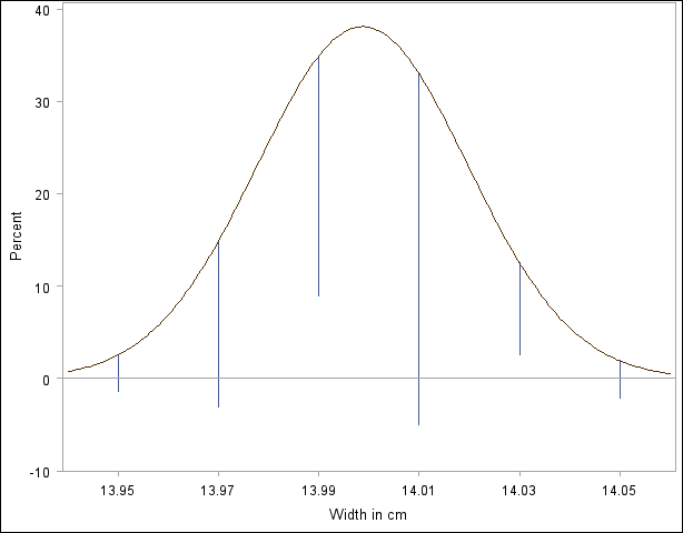

You can use the HANGING option only when exactly one fitted density curve is requested. A hanging histogram aligns the tops of the histogram bars (displayed as lines) with the fitted curve. The lines are positioned at the midpoints of the histogram bins. A hanging histogram is a goodness-of-fit diagnostic in the sense that the closer the lines are to the horizontal axis, the better the fit. Hanging histograms are discussed by Tukey (1977), Wainer (1974), and Velleman and Hoaglin (1981).

HOFFSET=value

specifies the offset, in percentage screen units, at both ends of the horizontal axis. You can use HOFFSET=0 to eliminate the default offset.

INTERBAR=value

specifies the space between histogram bars in percentage screen units. If both the INTERBAR= and BARWIDTH= options are specified, the INTERBAR= option takes precedence.

K=NORMAL | QUADRATIC | TRIANGULAR

specifies the kernel function (normal, quadratic, or triangular) used to compute a kernel density estimate. You can specify a list of values to request multiple estimates. You must enclose this option in parentheses after the KERNEL option. You can also use the K= kernel-option with the C= kernel-option, which specifies standardized bandwidths. If you specify more kernel functions than bandwidths, the procedure repeats the last bandwidth in the list for the remaining estimates. Similarly, if you specify more bandwidths than kernel functions, the procedure repeats the last kernel function for the remaining estimates. By default, K=NORMAL.

KERNEL<(kernel-options)>

superimposes kernel density estimates on the histogram. By default, the procedure uses the AMISE method to compute kernel density estimates. To request multiple kernel density estimates on the same histogram, specify a list of values for the C= kernel-option or K= kernel-option. Table 4.21 lists options you can specify with the KERNEL option. See the section Kernel Density Estimates for more information about kernel density estimates, and see Example 4.23.

LGRID=linetype

specifies the line type for the grid when a grid displays on the histogram. This option also creates a grid if the GRID option is not specified.

LOGNORMAL<(lognormal-options)>

displays fitted lognormal density curves on the histogram. The LOGNORMAL option can occur only once in a HISTOGRAM statement, but it can request any number of lognormal curves. The parameter $\text{[math]}$ must be less than the minimum data value. Use the THETA= lognormal-option to specify $\text{[math]}$ . By default, THETA=0. You can specify THETA=EST to request the maximum likelihood estimate for $\text{[math]}$ . Use the SIGMA= and ZETA= lognormal-options to specify $\text{[math]}$ and $\text{[math]}$ . By default, the procedure computes maximum likelihood estimates for $\text{[math]}$ and $\text{[math]}$ . Table 4.12 and Table 4.16 list options you can specify with the LOGNORMAL option. See the section Lognormal Distribution for details, and see Example 4.22 and Example 4.24 for examples using the LOGNORMAL option.

LOWER=value-list

specifies lower bounds for kernel density estimates requested with the KERNEL option. Enclose the LOWER= option in parentheses after the KERNEL option. If you specify more kernel estimates than lower bounds, the last lower bound is repeated for the remaining estimates. The default is a missing value, indicating no lower bounds for fitted kernel density curves.

MAXNBIN=n

limits the number of bins displayed in the comparative histogram. This option is useful when the scales or ranges of the data distributions differ greatly from cell to cell. By default, the bin size and midpoints are determined for the key cell, and then the midpoint list is extended to accommodate the data ranges for the remaining cells. However, if the cell scales differ considerably, the resulting number of bins can be so great that each cell histogram is scaled into a narrow region. By using MAXNBIN= to limit the number of bins, you can narrow the window about the data distribution in the key cell. This option is not available unless you specify the CLASS statement. The MAXNBIN= option is an alternative to the MAXSIGMAS= option.

MAXSIGMAS=value

limits the number of bins displayed in the comparative histogram to a range of value standard deviations (of the data in the key cell) above and below the mean of the data in the key cell. This option is useful when the scales or ranges of the data distributions differ greatly from cell to cell. By default, the bin size and midpoints are determined for the key cell, and then the midpoint list is extended to accommodate the data ranges for the remaining cells. However, if the cell scales differ considerably, the resulting number of bins can be so great that each cell histogram is scaled into a narrow region. By using MAXSIGMAS= to limit the number of bins, you can narrow the window that surrounds the data distribution in the key cell. This option is not available unless you specify the CLASS statement.

MIDPERCENTS

requests a table listing the midpoints and percentage of observations in each histogram interval. If you specify MIDPERCENTS in parentheses after a density estimate option, the procedure displays a table that lists the midpoints, the observed percentage of observations, and the estimated percentage of the population in each interval (estimated from the fitted distribution). See Example 4.18.

MIDPOINTS=values | KEY | UNIFORM

specifies how to determine the midpoints for the histogram intervals, where values determines the width of the histogram bars as the difference between consecutive midpoints. The procedure uses the same values for all variables.

The range of midpoints, extended at each end by half of the bar width, must cover the range of the data. For example, if you specify

   midpoints=2 to 10 by 0.5

then all of the observations should fall between 1.75 and 10.25. You must use evenly spaced midpoints listed in increasing order.

KEY: determines the midpoints for the data in the key cell. The initial number of midpoints is based on the number of observations in the key cell that use the method of Terrell and Scott (1985). The procedure extends the midpoint list for the key cell in either direction as necessary until it spans the data in the remaining cells.
UNIFORM: determines the midpoints by using all the observations as if there were no cells. In other words, the number of midpoints is based on the total sample size by using the method of Terrell and Scott (1985).

Neither KEY nor UNIFORM apply unless you use the CLASS statement. By default, if you use a CLASS statement, MIDPOINTS=KEY; however, if the key cell is empty then MIDPOINTS=UNIFORM. Otherwise, the procedure computes the midpoints by using an algorithm (Terrell and Scott; 1985) that is primarily applicable to continuous data that are approximately normally distributed.

MU=value-list

specifies the parameter $\text{[math]}$ for normal density curves requested with the NORMAL option. Enclose the MU= option in parentheses after the NORMAL option. By default, or if you specify the value EST, the procedure uses the sample mean for $\text{[math]}$ .

NENDPOINTS= $\text{[math]}$

uses histogram interval endpoints as the tick mark values for the horizontal axis and determines the number of bins.

NMIDPOINTS= $\text{[math]}$

specifies the number of histogram intervals.

NOBARS

suppresses drawing of histogram bars, which is useful for viewing fitted curves only.

NOPLOT

NOCHART

suppresses the creation of a plot. Use this option when you only want to tabulate summary statistics for a fitted density or create an OUTHISTOGRAM= data set.

NOPRINT

suppresses tables summarizing the fitted curve. Enclose the NOPRINT option in parentheses following the distribution option.

NORMAL<(normal-options)>

displays fitted normal density curves on the histogram. The NORMAL option can occur only once in a HISTOGRAM statement, but it can request any number of normal curves. Use the MU= and SIGMA= normal-options to specify $\text{[math]}$ and $\text{[math]}$ . By default, the procedure uses the sample mean and sample standard deviation for $\text{[math]}$ and $\text{[math]}$ . Table 4.12 and Table 4.17 list options you can specify with the NORMAL option. See the section Normal Distribution for details, and see Example 4.19 for an example that uses the NORMAL option.

NOTABCONTENTS

suppresses the table of contents entries for tables produced by the HISTOGRAM statement.

OUTHISTOGRAM=SAS-data-set

OUTHIST=SAS-data-set

creates a SAS data set that contains information about histogram intervals. Specifically, the data set contains the midpoints of the histogram intervals (or the lower endpoints of the intervals if you specify the ENDPOINTS option), the observed percentage of observations in each interval, and the estimated percentage of observations in each interval (estimated from each of the specified fitted curves).

PERCENTS=values

PERCENT=values

specifies a list of percents for which quantiles calculated from the data and quantiles estimated from the fitted curve are tabulated. The percents must be between 0 and 100. Enclose the PERCENTS= option in parentheses after the curve option. The default percents are 1, 5, 10, 25, 50, 75, 90, 95, and 99.

PFILL=pattern

specifies a pattern used to fill the bars of the histograms (or the areas under a fitted curve if you also specify the FILL option) when producing traditional graphics. See the entries for the CFILL= and FILL options for additional details. Refer to SAS/GRAPH: Reference for a list of pattern values. The option does not apply to ODS Graphics output.

RTINCLUDE

includes the right endpoint of each histogram interval in that interval. By default, the left endpoint is included in the histogram interval.

SB<( $\text{[math]}$ -options)>

displays fitted Johnson $\text{[math]}$ density curves on the histogram. The SB option can occur only once in a HISTOGRAM statement, but it can request any number of Johnson $\text{[math]}$ curves. Use the THETA= and SIGMA= normal-options to specify $\text{[math]}$ and $\text{[math]}$ . By default, the procedure computes maximum likelihood estimates of $\text{[math]}$ and $\text{[math]}$ . Table 4.12 and Table 4.18 list options you can specify with the SB option. See the section Johnson $\text{[math]}$ Distribution for details.

SIGMA=value-list

specifies the parameter $\text{[math]}$ for the fitted density curve when you request the BETA, EXPONENTIAL, GAMMA, LOGNORMAL, NORMAL, SB, SU, or WEIBULL options.

See Table 4.24 for a summary of how to use the SIGMA= option. You must enclose this option in parentheses after the density curve option. You can specify the value EST to request a maximum likelihood estimate for $\text{[math]}$ .

Table 4.24 Uses of the SIGMA= Option
Distribution Keyword	SIGMA= Specifies	Default Value	Alias
BETA	scale parameter $\text{[math]}$	1	SCALE=
EXPONENTIAL	scale parameter $\text{[math]}$	maximum likelihood estimate	SCALE=
GAMMA	scale parameter $\text{[math]}$	maximum likelihood estimate	SCALE=
LOGNORMAL	shape parameter $\text{[math]}$	maximum likelihood estimate	SHAPE=
NORMAL	scale parameter $\text{[math]}$	standard deviation
SB	scale parameter $\text{[math]}$	1	SCALE=
SU	scale parameter $\text{[math]}$	percentile-based estimate
WEIBULL	scale parameter $\text{[math]}$	maximum likelihood estimate	SCALE=

SU<( $\text{[math]}$ -options)>

displays fitted Johnson $\text{[math]}$ density curves on the histogram. The SU option can occur only once in a HISTOGRAM statement, but it can request any number of Johnson $\text{[math]}$ curves. Use the THETA= and SIGMA= normal-options to specify $\text{[math]}$ and $\text{[math]}$ . By default, the procedure computes maximum likelihood estimates of $\text{[math]}$ and $\text{[math]}$ . Table 4.12 and Table 4.19 list options you can specify with the SU option. See the section Johnson $\text{[math]}$ Distribution for details.

THETA=value-list

THRESHOLD= value-list

specifies the lower threshold parameter $\text{[math]}$ for curves requested with the BETA, EXPONENTIAL, GAMMA, LOGNORMAL, SB, SU, and WEIBULL options. Enclose the THETA= option in parentheses after the curve option. By default, THETA=0. If you specify the value EST, an estimate is computed for $\text{[math]}$ .

UPPER=value-list

specifies upper bounds for kernel density estimates requested with the KERNEL option. Enclose the UPPER= option in parentheses after the KERNEL option. If you specify more kernel estimates than upper bounds, the last upper bound is repeated for the remaining estimates. The default is a missing value, indicating no upper bounds for fitted kernel density curves.

VOFFSET=value

specifies the offset, in percentage screen units, at the upper end of the vertical axis.

VSCALE=COUNT | PERCENT | PROPORTION

specifies the scale of the vertical axis for a histogram. The value COUNT requests the data be scaled in units of the number of observations per data unit. The value PERCENT requests the data be scaled in units of percent of observations per data unit. The value PROPORTION requests the data be scaled in units of proportion of observations per data unit. The default is PERCENT.

WBARLINE=n

specifies the width of bar outlines when producing traditional graphics. The option does not apply to ODS Graphics output.

WEIBULL<(Weibull-options)>

displays fitted Weibull density curves on the histogram. The WEIBULL option can occur only once in a HISTOGRAM statement, but it can request any number of Weibull curves. The parameter $\text{[math]}$ must be less than the minimum data value. Use the THETA= Weibull-option to specify $\text{[math]}$ . By default, THETA=0. You can specify THETA=EST to request the maximum likelihood estimate for $\text{[math]}$ . Use the C= and SIGMA= Weibull-options to specify the shape parameter $\text{[math]}$ and the scale parameter $\text{[math]}$ . By default, the procedure computes the maximum likelihood estimates for $\text{[math]}$ and $\text{[math]}$ . Table 4.12 and Table 4.20 list options you can specify with the WEIBULL option. See the section Weibull Distribution for details, and see Example 4.22 for an example that uses the WEIBULL option.

PROC UNIVARIATE calculates the maximum likelihood estimate of $\text{[math]}$ iteratively by using the Newton-Raphson approximation. See also the C=, SIGMA=, and THETA= Weibull-options.

WGRID=n

specifies the line thickness for the grid when producing traditional graphics. The option does not apply to ODS Graphics output.

ZETA= value-list

specifies a value for the scale parameter $\text{[math]}$ for lognormal density curves requested with the LOGNORMAL option. Enclose the ZETA= lognormal-option in parentheses after the LOGNORMAL option. By default, or if you specify the value EST, the procedure calculates a maximum likelihood estimate for $\text{[math]}$ . You can specify the SCALE= option as an alias for the ZETA= option.

Top of Page