The HPSUMMARY Procedure

Keywords and Formulas
Simple Statistics
The HPSUMMARY procedure uses a standardized set of keywords to refer to statistics. You specify these keywords in SAS statements to request the statistics to be displayed or stored in an output data set.
In the following notation, summation is over observations that contain nonmissing values of the analyzed variable and, except where shown, over nonmissing weights and frequencies of one or more:

-
is the nonmissing value of the analyzed variable for observation i. 
-
is the frequency that is associated with if you use a FREQ
statement. If you omit the FREQ statement, then  for all i.

-
is the weight that is associated with if you use a WEIGHT
statement. The HPSUMMARY procedure automatically excludes the values of with missing weights from the analysis.
By default, the HPSUMMARY procedure treats a negative weight as if it is equal to 0. However, if you use the EXCLNPWGT option in the PROC HPSUMMARY statement, then the procedure also excludes those values of with nonpositive weights.
If you omit the WEIGHT statement, then
 for all i.
- n
-
is the number of nonmissing values of,  . If you use the EXCLNPWGT option and the WEIGHT statement, then n is the number of nonmissing values with positive weights.

-
is the mean![\[ \left.\sum w_ i x_ i\middle /\sum w_ i\right. \]](images/prochp_hpsummary0052.png)

-
is the variance![\[ \frac{1}{d} \sum w_ i (x_ i - \bar{x})^2 \]](images/prochp_hpsummary0054.png)
where d is the variance divisor (the VARDEF= option) that you specify in the PROC HPSUMMARY statement. Valid values are as follows:
Table 10.9: (continued)
When VARDEF=
d equals
N
n
DF

WEIGHT | WGT

WDF

The default is DF.

-
is the standardized variable![\[ (x_ i - \bar{x}) / s \]](images/prochp_hpsummary0056.png)
PROC HPSUMMARY calculates the following simple statistics:
-
number of missing values
-
number of nonmissing values
-
number of observations
-
sum of weights
-
mean
-
sum
-
extreme values
-
minimum
-
maximum
-
range
-
uncorrected sum of squares
-
corrected sum of squares
-
variance
-
standard deviation
-
standard error of the mean
-
coefficient of variation
-
skewness
-
kurtosis
-
confidence limits of the mean
-
median
-
mode
-
percentiles/deciles/quartiles
-
t test for mean=0
The standard keywords and formulas for each statistic follow. Some formulas use keywords to designate the corresponding statistic.
Descriptive Statistics
The keywords for descriptive statistics are as follows:
- CSS
-
is the sum of squares corrected for the mean, computed as![\[ \sum w_ i (x_ i - \bar{x})^2 \]](images/prochp_hpsummary0057.png)
- CV
-
is the percent coefficient of variation, computed as![\[ (100s) / \bar{x} \]](images/prochp_hpsummary0058.png)
- KURTOSIS | KURT
-
is the kurtosis, which measures heaviness of tails. When VARDEF= DF, the kurtosis is computed as![\[ c_{4_ n} \sum z_ i^4 - \frac{3 \left( n-1 \right)^2}{\left( n-2 \right) \left( n-3 \right)} \]](images/prochp_hpsummary0059.png)
where
 is
is 
When VARDEF=N, the kurtosis is computed as
![\[ \frac{1}{n} \sum z_ i^4 - 3 \]](images/prochp_hpsummary0062.png)
The formula is invariant under the transformation
 ,
,  . When you use VARDEF=WDF or VARDEF=WEIGHT, the kurtosis is set to missing.
- MAX
-
is the maximum value of.
- MEAN
-
is the arithmetic mean.
- MIN
-
is the minimum value of.
- MODE
-
is the most frequent value of.
Note: When QMETHOD=P2, PROC HPSUMMARY does not compute MODE.
- N
-
is the number of values that are not missing. Observations with  and equal to missing or
  (when you use the EXCLNPWGT
option) are excluded from the analysis and are not included in the calculation of N.
(when you use the EXCLNPWGT
option) are excluded from the analysis and are not included in the calculation of N.
- NMISS
-
is the number of values that are missing. Observations with and equal to missing or (when you use the EXCLNPWGT option) are excluded from the analysis and are not included in the calculation of NMISS.
- NOBS
-
is the total number of observations and is calculated as the sum of N and NMISS. However, if you use the WEIGHT statement, then NOBS is calculated as the sum of N, NMISS, and the number of observations excluded because of missing or nonpositive weights. - RANGE
-
is the range and is calculated as the difference between maximum value and minimum value. - SKEWNESS | SKEW
-
is skewness, which measures the tendency of the deviations to be larger in one direction than in the other. When VARDEF=DF, the skewness is computed as![\[ c_{3_ n} \sum z_ i^3 \]](images/prochp_hpsummary0067.png)
where
 is
is  .
.
When VARDEF=N, the skewness is computed as
![\[ \frac{1}{n} \sum z_ i^3 \]](images/prochp_hpsummary0070.png)
The formula is invariant under the transformation
, . When you use VARDEF=WDF or VARDEF=WEIGHT, the skewness is set to missing.
- STDDEV | STD
-
is the standard deviation s and is computed as the square root of the variance,.
- STDERR | STDMEAN
-
is the standard error of the mean, computed as![\[ \frac{s}{\sqrt {\sum w_ i}} \]](images/prochp_hpsummary0071.png)
when VARDEF=DF, which is the default. Otherwise, STDERR is set to missing.
- SUM
-
is the sum, computed as![\[ \sum w_ i x_ i \]](images/prochp_hpsummary0072.png)
- SUMWGT
-
is the sum of the weights, W, computed as![\[ \sum w_ i \]](images/prochp_hpsummary0073.png)
- USS
-
is the uncorrected sum of squares, computed as![\[ \sum w_ i x_ i^2 \]](images/prochp_hpsummary0074.png)
- VAR
-
is the variance.
Quantile and Related Statistics
The keywords for quantiles and related statistics are as follows:
- MEDIAN
-
is the middle value. - Pn
-
is the nth percentile. For example, P1 is the first percentile, P5 is the fifth percentile, P50 is the 50th percentile, and P99 is the 99th percentile. - Q1
-
is the lower quartile (25th percentile). - Q3
-
is the upper quartile (75th percentile). - QRANGE
-
is interquartile range and is calculated as![\[ Q_3 - Q_1 \]](images/prochp_hpsummary0075.png)
You use the QNTLDEF=
option to specify the method that the HPSUMMARY procedure uses to compute percentiles. Let n be the number of nonmissing values for a variable, and let  represent the ordered values of the variable such that
  is the smallest value,
  is the next smallest value, and
  is the largest value. For the tth percentile between 0 and 1, let
  . Then define j as the integer part of
  and g as the fractional part of or
  , so that
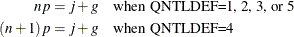
Here, QNTLDEF= specifies the method that the procedure uses to compute the tth percentile, as shown in Table 10.10.
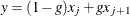
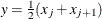
When you use the WEIGHT statement, the tth percentile is computed as
![\[ y = \begin{cases} \frac{1}{2} \left( x_ i + x_{i+1} \right) & \mbox{if} \displaystyle \sum _{j=1}^ i w_ j = pW \\ x_{i+1} & \mbox{if} \displaystyle \sum _{j=1}^ i w_ j < pW < \displaystyle \sum _{j=1}^{i+1} w_ j \end{cases} \]](images/prochp_hpsummary0084.png)
where  is the weight associated with and
  is the sum of the weights. When the observations have identical weights, the weighted percentiles are the same as the unweighted
percentiles with QNTLDEF=5.
is the sum of the weights. When the observations have identical weights, the weighted percentiles are the same as the unweighted
percentiles with QNTLDEF=5.
Table 10.10: Methods for Computing Quantile Statistics
|
QNTLDEF= |
Description |
Formula |
|
|---|---|---|---|
|
1 |
Weighted average at |
|
|
|
where |
|||
|
2 |
Observation numbered closest to |
|
if |
|
|
if |
||
|
|
if |
||
|
where i is the integer part of |
|||
|
3 |
Empirical distribution function |
|
if |
|
|
if |
||
|
4 |
Weighted average aimed at |
|
|
|
where |
|||
|
5 |
Empirical distribution function with averaging |
|
if |
|
|
if |
||


Hypothesis Testing Statistics
The keywords for hypothesis testing statistics are as follows:
- T
-
is the Student’s t statistic to test the null hypothesis that the population mean is equal to and is calculated as
![\[ \frac{\bar{x} - \mu _0}{\left.s\middle /\sqrt {\sum w_ i}\right.} \]](images/prochp_hpsummary0101.png)
By default,
is equal to zero. You must use VARDEF=
DF, which is the default variance divisor; otherwise T is set to missing.
By default, when you use a WEIGHT statement, the procedure counts the
values with nonpositive weights in the degrees of freedom. Use the EXCLNPWGT
option in the PROC HPSUMMARY
statement to exclude values with nonpositive weights.
- PROBT | PRT
-
is the two-tailed p-value for the Student’s t statistic, T, with degrees of freedom. This value is the probability under the null hypothesis of obtaining a more extreme value of T than is
observed in this sample.
Confidence Limits for the Mean
The keywords for confidence limits are as follows:
- CLM
-
is the two-sided confidence limit for the mean. A two-sided percent confidence interval for the mean has upper and lower limits
![\[ \bar{x} \pm t_{(1-\alpha /2;\, n-1)} \frac{s}{\sqrt {\sum w_ i}} \]](images/prochp_hpsummary0102.png)
where s is
 ,
,  is the
  critical value of the Student’s t statistic with
  degrees of freedom, and
  is the value of the ALPHA=
option which by default is 0.05. Unless you use VARDEF=
DF (which is the default variance divisor), CLM is set to missing.
is the value of the ALPHA=
option which by default is 0.05. Unless you use VARDEF=
DF (which is the default variance divisor), CLM is set to missing.
- LCLM
-
is the one-sided confidence limit below the mean. The one-sided percent confidence interval for the mean has the lower limit
![\[ \bar{x} - t_{(1-\alpha ;\, n-1)} \frac{s}{\sqrt {\sum w_ i}} \]](images/prochp_hpsummary0106.png)
Unless you use VARDEF=DF (which is the default variance divisor), LCLM is set to missing.
- UCLM
-
is the one-sided confidence limit above the mean. The one-sided percent confidence interval for the mean has the upper limit
![\[ \bar{x} + t_{(1-\alpha ;\, n-1)} \frac{s}{\sqrt {\sum w_ i}} \]](images/prochp_hpsummary0107.png)
Unless you use VARDEF=DF (which is the default variance divisor), UCLM is set to missing.
Data Requirements for the HPSUMMARY Procedure
The following are the minimal data requirements to compute unweighted statistics and do not describe recommended sample sizes. Statistics are reported as missing if VARDEF =DF (the default) and the following requirements are not met:
-
N and NMISS are computed regardless of the number of missing or nonmissing observations.
-
SUM, MEAN, MAX, MIN, RANGE, USS, and CSS require at least one nonmissing observation.
-
VAR, STD, STDERR, CV, T, PRT, and PROBT require at least two nonmissing observations.
-
SKEWNESS requires at least three nonmissing observations.
-
KURTOSIS requires at least four nonmissing observations.
-
SKEWNESS, KURTOSIS, T, PROBT, and PRT require that STD is greater than zero.
-
CV requires that MEAN is not equal to zero.
-
CLM, LCLM, UCLM, STDERR, T, PRT, and PROBT require that VARDEF=DF.