Example 3.8 Project Cost Control
Cost control and accounting are important aspects of project management. Cost data for a project may be associated with activities or groups of activities, or with resources, such as personnel or equipment. For example, consider a project that consists of several subprojects, each of which is contracted to a different company. From the contracting company’s point of view, each subproject can be treated as one cost item; all the company needs to know is how much each subproject is going to cost. On the other hand, another project may contain several activities, each of which requires two types of labor, skilled and unskilled. The cost for each activity in the project may have to be computed on the basis of how much skilled or unskilled labor that activity uses. In this case, activity and project costs are determined from the resources used. Further, for any project, there may be several ways in which costs need to be summarized and accounted for. In addition to determining the cost of each individual activity, you may want to determine periodic budgets for different departments that are involved with the project or compare the actual costs that were incurred with the budgeted costs.
It is easy to set up cost accounting systems using the output data sets produced by PROC CPM, whether costs are associated with activities or with resources. In fact, you can even treat cost as a consumable resource if you can estimate the cost per day for each of the activities (see
Chapter 4,
The CPM Procedure,
for details about resource allocation and types of resources). This example illustrates such a method for monitoring costs and shows how you can compute some of the standard cost performance measures used in project management.
The following three measures can be used to determine if a project is running on schedule and within budget (see Moder, Phillips, and Davis 1983, for a detailed discussion on project cost control):
Actual cost of work performed (ACWP) is the actual cost expended to perform the work accomplished in a given period of time.
Budgeted cost of work performed (BCWP) is the budgeted cost of the work completed in a given period of time.
Budgeted cost of work scheduled (BCWS) is the budgeted cost of the work scheduled to be accomplished in a given period of time (if a baseline schedule were followed).
Consider the survey example described earlier in this chapter. Suppose that it is possible to estimate the cost per day for each activity in the project. The following data set survcost contains the project data (activity, succ1–succ3, id, duration) and a variable named cost containing the cost per day in dollars. In order to compute the BCWS for the project, you need to establish a baseline schedule. Suppose the early start schedule computed by PROC CPM is chosen as the baseline schedule. The Resource data set costavl establishes cost as a consumable resource, so that the CPM procedure can be used to accumulate costs (using the CUMUSAGE option).
The following program invokes PROC CPM with the RESOURCE statement and saves the Usage data set in survrout. The variable ecost in this Usage data set contains the cumulative expense incurred for the baseline schedule; this is the same as the budgeted cost of work scheduled (or BCWS) saved in the data set basecost.
data survcost;
   format id $20. activity $8. succ1-succ3 $8. ;
   input id & activity & duration succ1 & succ2 & succ3 & cost;
   datalines;
Plan Survey           plan sur   4 hire per  design q  .        300
Hire Personnel        hire per   5 trn per   .         .        350
Design Questionnaire  design q   3 trn per   select h  print q  100
Train Personnel       trn per    3 cond sur  .         .        500
Select Households     select h   3 cond sur  .         .        300
Print Questionnaire   print q    4 cond sur  .         .        250
Conduct Survey        cond sur  10 analyze   .         .        200
Analyze Results       analyze    6 .         .         .        500
;

data holidata;
   format hol date7.;
   hol = '4jul03'd;
   run;

data costavl;
   input per & date7. otype $ cost;
   format per date7.;
   datalines;
.       restype   2
1jul03  reslevel  12000
;
proc cpm date='1jul03'd interval=weekday
         data=survcost resin=costavl   holidata=holidata
         out=sched     resout=survrout;
   activity   activity;
   successor  succ1-succ3;
   duration   duration;
   holiday    hol;
   id         id;
   resource   cost / period  = per
                     obstype = otype cumusage;
   run;
data basecost (keep = _time_ bcws);
   set survrout;
   bcws = ecost;
   run;
Suppose that the project started as planned on July 1, 2003, but some of the activities took longer than planned and some of the cost estimates were found to be incorrect. The following data set, actual, contains updated information: the variables as and af contain the actual start and finish times of the activities that have been completed or are in progress. The variable actcost contains the revised cost per day for each activity. The following program combines this information with the existing project data and saves the result in the data set update, displayed in Output 3.8.1. The Resource data set costavl2 (also displayed in Output 3.8.1) defines cost and actcost as consumable resources.
data actual;
   format id $20. ;
   input id & as & date9. af & date9. actcost;
   format as af date7.;
   datalines;
Plan Survey            1JUL03   8JUL03   275
Hire Personnel         9JUL03  15JUL03   350
Design Questionnaire  10JUL03  14JUL03   150
Train Personnel       16JUL03  17JUL03   800
Select Households     15JUL03  17JUL03   450
Print Questionnaire   15JUL03  18JUL03   250
Conduct Survey        21JUL03   .        200
;

data work.update;
   merge survcost actual;
   run;

data costavl2;
   input per & date7. otype $ cost actcost;
   format per date7.;
   datalines;
.       restype   2      2
1jul03  reslevel  12000  12000
;
title 'Activity Data Set UPDATE';
proc print data=work.update;
   run;

title 'Resource Data Set COSTAVL2';
proc print data=costavl2;
   run;
| Activity Data Set UPDATE |
| Obs | id | activity | succ1 | succ2 | succ3 | duration | cost | as | af | actcost |
|---|---|---|---|---|---|---|---|---|---|---|
| 1 | Plan Survey | plan sur | hire per | design q | 4 | 300 | 01JUL03 | 08JUL03 | 275 | |
| 2 | Hire Personnel | hire per | trn per | 5 | 350 | 09JUL03 | 15JUL03 | 350 | ||
| 3 | Design Questionnaire | design q | trn per | select h | print q | 3 | 100 | 10JUL03 | 14JUL03 | 150 |
| 4 | Train Personnel | trn per | cond sur | 3 | 500 | 16JUL03 | 17JUL03 | 800 | ||
| 5 | Select Households | select h | cond sur | 3 | 300 | 15JUL03 | 17JUL03 | 450 | ||
| 6 | Print Questionnaire | print q | cond sur | 4 | 250 | 15JUL03 | 18JUL03 | 250 | ||
| 7 | Conduct Survey | cond sur | analyze | 10 | 200 | 21JUL03 | . | 200 | ||
| 8 | Analyze Results | analyze | 6 | 500 | . | . | . |
Next, PROC CPM is used to revise the schedule by using the ACTUAL statement to specify the actual start and finish times and the RESOURCE statement to specify both the budgeted and the actual costs. The resulting schedule is saved in the data set updsched (displayed in Output 3.8.2) and the budgeted and the actual cumulative costs of the project (until the current date) are saved in the data set updtrout. These cumulative costs represent the budgeted cost of work performed (BCWP) and the actual cost of work performed (ACWP), respectively, and are saved in the data set updtcost. The two data sets basecost and updtcost are then merged to create a data set that contains the three measures: bcws, bcwp, and acwp. The resulting data set is displayed in Output 3.8.3.
proc cpm date='1jul03'd interval=weekday
         data=work.update    resin=costavl2
         out=updsched   resout=updtrout
         holidata=holidata;
   activity   activity;
   successor  succ1-succ3;
   duration   duration;
   holiday    hol;
   id         id;
   resource   cost actcost / per     = per
                             obstype = otype
                             maxdate = '21jul03'd cumusage;
   actual / a_start=as a_finish=af;
   run;
title 'Updated Schedule: Data Set UPDSCHED';
proc print data=updsched;
   run;
data updtcost (keep = _time_ bcwp acwp);
   set updtrout;
   bcwp = ecost;
   acwp = eactcost;
   run;

/* Create a combined data set to contain the BCWS, BCWP, ACWP */
/* per day and the cumulative values for these costs.         */
data costs;
   merge basecost updtcost;
   run;
title 'BCWS, BCWP, and ACWP';
proc print data=costs;
   run;
| Updated Schedule: Data Set UPDSCHED |
| Obs | activity | succ1 | succ2 | succ3 | duration | STATUS | A_DUR | id | cost | actcost | A_START | A_FINISH | S_START | S_FINISH | E_START | E_FINISH | L_START | L_FINISH |
|---|---|---|---|---|---|---|---|---|---|---|---|---|---|---|---|---|---|---|
| 1 | plan sur | hire per | design q | 4 | Completed | 5 | Plan Survey | 300 | 275 | 01JUL03 | 08JUL03 | 01JUL03 | 08JUL03 | 01JUL03 | 08JUL03 | 01JUL03 | 08JUL03 | |
| 2 | hire per | trn per | 5 | Completed | 5 | Hire Personnel | 350 | 350 | 09JUL03 | 15JUL03 | 09JUL03 | 15JUL03 | 09JUL03 | 15JUL03 | 09JUL03 | 15JUL03 | ||
| 3 | design q | trn per | select h | print q | 3 | Completed | 3 | Design Questionnaire | 100 | 150 | 10JUL03 | 14JUL03 | 10JUL03 | 14JUL03 | 10JUL03 | 14JUL03 | 10JUL03 | 14JUL03 |
| 4 | trn per | cond sur | 3 | Completed | 2 | Train Personnel | 500 | 800 | 16JUL03 | 17JUL03 | 16JUL03 | 17JUL03 | 16JUL03 | 17JUL03 | 16JUL03 | 17JUL03 | ||
| 5 | select h | cond sur | 3 | Completed | 3 | Select Households | 300 | 450 | 15JUL03 | 17JUL03 | 15JUL03 | 17JUL03 | 15JUL03 | 17JUL03 | 15JUL03 | 17JUL03 | ||
| 6 | print q | cond sur | 4 | Completed | 4 | Print Questionnaire | 250 | 250 | 15JUL03 | 18JUL03 | 15JUL03 | 18JUL03 | 15JUL03 | 18JUL03 | 15JUL03 | 18JUL03 | ||
| 7 | cond sur | analyze | 10 | In Progress | . | Conduct Survey | 200 | 200 | 21JUL03 | . | 21JUL03 | 01AUG03 | 21JUL03 | 01AUG03 | 21JUL03 | 01AUG03 | ||
| 8 | analyze | 6 | Pending | . | Analyze Results | 500 | . | . | . | 04AUG03 | 11AUG03 | 04AUG03 | 11AUG03 | 04AUG03 | 11AUG03 |
| BCWS, BCWP, and ACWP |
| Obs | _TIME_ | bcws | bcwp | acwp |
|---|---|---|---|---|
| 1 | 01JUL03 | 0 | 0 | 0 |
| 2 | 02JUL03 | 300 | 300 | 275 |
| 3 | 03JUL03 | 600 | 600 | 550 |
| 4 | 07JUL03 | 900 | 900 | 825 |
| 5 | 08JUL03 | 1200 | 1200 | 1100 |
| 6 | 09JUL03 | 1650 | 1500 | 1375 |
| 7 | 10JUL03 | 2100 | 1850 | 1725 |
| 8 | 11JUL03 | 2550 | 2300 | 2225 |
| 9 | 14JUL03 | 3450 | 2750 | 2725 |
| 10 | 15JUL03 | 4350 | 3200 | 3225 |
| 11 | 16JUL03 | 5400 | 4100 | 4275 |
| 12 | 17JUL03 | 6150 | 5150 | 5775 |
| 13 | 18JUL03 | 6650 | 6200 | 7275 |
| 14 | 21JUL03 | 6850 | 6450 | 7525 |
| 15 | 22JUL03 | 7050 | . | . |
| 16 | 23JUL03 | 7250 | . | . |
| 17 | 24JUL03 | 7450 | . | . |
| 18 | 25JUL03 | 7650 | . | . |
| 19 | 28JUL03 | 7850 | . | . |
| 20 | 29JUL03 | 8050 | . | . |
| 21 | 30JUL03 | 8250 | . | . |
| 22 | 31JUL03 | 8450 | . | . |
| 23 | 01AUG03 | 8650 | . | . |
| 24 | 04AUG03 | 9150 | . | . |
| 25 | 05AUG03 | 9650 | . | . |
| 26 | 06AUG03 | 10150 | . | . |
| 27 | 07AUG03 | 10650 | . | . |
| 28 | 08AUG03 | 11150 | . | . |
| 29 | 11AUG03 | 11650 | . | . |
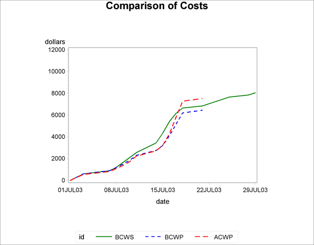
The data set costs, containing the required cost information, is then used as input to PROC GPLOT to produce a plot of the three cumulative cost measures. The plot is shown in Output 3.8.4.
Note: BCWS, BCWP, and ACWP are three of the cost measures used as part of Earned Value Analysis, which is an important component of the Cost/Schedule Control Systems Criteria (referred to as C/SCSC) that was established in 1967 by the Department of Defense (DOD) to standardize the reporting of cost and schedule performance on major contracts. Refer to Fleming (1988) for a detailed discussion of C/SCSC. Similar methods, such as the ones described in this example, can be used to calculate all the relevant measures for analyzing cost and schedule performance.
   /* Plot the cumulative costs */
   data costplot (keep=date dollars id);
      set costs;
      format date date7.;
      date = _time_;
      if bcws ^= . then do;
         dollars = BCWS; id = 1; output;
         end;
      if bcwp ^= . then do;
         dollars = BCWP; id = 2; output;
         end;
      if acwp ^= . then do;
         dollars = ACWP; id = 3; output;
         end;
      run;
legend1 frame
        value=(c=black j=l 'BCWS' 'BCWP' 'ACWP')
        label=(c=black);

axis1 width=2
      order=('1jul03'd to '1aug03'd by week)
      length=60 pct
      value=(c=black)
      label=(c=black);

axis2 width=2
      order=(0 to 12000 by 2000)
      length = 55 pct
      value=(c=black)
      label=(c=black);

symbol1 i=join v=none c=green  w=4 l=1;
symbol2 i=join v=none c=blue   w=4 l=2;
symbol3 i=join v=none c=red    w=4 l=3;
title c=black h=2.5 'Comparison of Costs';

proc gplot data=costplot;
   plot dollars * date = id / legend=legend1
                              haxis=axis1
                              vaxis=axis2;
   run;