The Mixed Integer Linear Programming Solver

Consider the classic facility location problem. Given a set L of customer locations and a set F of candidate facility sites, you must decide on which sites to build facilities and assign coverage of customer demand to
these sites so as to minimize cost. All customer demand ![]() must be satisfied, and each facility has a demand capacity limit C. The total cost is the sum of the distances
must be satisfied, and each facility has a demand capacity limit C. The total cost is the sum of the distances ![]() between facility j and its assigned customer i, plus a fixed charge
between facility j and its assigned customer i, plus a fixed charge ![]() for building a facility at site j. Let
for building a facility at site j. Let ![]() represent choosing site j to build a facility, and 0 otherwise. Also, let
represent choosing site j to build a facility, and 0 otherwise. Also, let ![]() represent the assignment of customer i to facility j, and 0 otherwise. This model can be formulated as the following integer linear program:
represent the assignment of customer i to facility j, and 0 otherwise. This model can be formulated as the following integer linear program:
![\[ \begin{array}{llllll} \min & \displaystyle \sum _{i \in L} \displaystyle \sum _{j \in F} c_{ij} x_{ij} + \displaystyle \sum _{j \in F} f_ j y_ j \\ \mr {s.t.} & \displaystyle \sum _{j \in F} x_{ij} & = & 1 & \forall i \in L & \mr {(assign\_ def)} \\ & x_{ij} & \leq & y_ j & \forall i \in L, j \in F & \mr {(link)}\\ & \displaystyle \sum _{i \in L} d_ i x_{ij} & \leq & Cy_ j & \forall j \in F & \mr {(capacity)} \\ & x_{ij} \in \{ 0,1\} & & & \forall i \in L, j \in F \\ & y_{j} \in \{ 0,1\} & & & \forall j \in F \end{array} \]](images/ormpug_milpsolver0080.png)
Constraint (assign_def) ensures that each customer is assigned to exactly one site. Constraint (link) forces a facility to be built if any customer has been assigned to that facility. Finally, constraint (capacity) enforces the capacity limit at each site.
Consider also a variation of this same problem where there is no cost for building a facility. This problem is typically easier to solve than the original problem. For this variant, let the objective be
First, construct a random instance of this problem by using the following DATA steps:
title 'Facility Location Problem';
%let NumCustomers  = 50;
%let NumSites      = 10;
%let SiteCapacity  = 35;
%let MaxDemand     = 10;
%let xmax          = 200;
%let ymax          = 100;
%let seed          = 938;

/* generate random customer locations */
data cdata(drop=i);
   length name $8;
   do i = 1 to &NumCustomers;
      name = compress('C'||put(i,best.));
      x = ranuni(&seed) * &xmax;
      y = ranuni(&seed) * &ymax;
      demand = ranuni(&seed) * &MaxDemand;
      output;
   end;
run;

/* generate random site locations and fixed charge */
data sdata(drop=i);
   length name $8;
   do i = 1 to &NumSites;
      name = compress('SITE'||put(i,best.));
      x = ranuni(&seed) * &xmax;
      y = ranuni(&seed) * &ymax;
      fixed_charge = 30 * (abs(&xmax/2-x) + abs(&ymax/2-y));
      output;
   end;
run;
The following PROC OPTMODEL statements first generate and solve the model with the no-fixed-charge variant of the cost function. Next, they solve the fixed-charge model. Note that the solution to the model with no fixed charge is feasible for the fixed-charge model and should provide a good starting point for the MILP solver. Use the PRIMALIN option to provide an incumbent solution (warm start).
proc optmodel;
   set <str> CUSTOMERS;
   set <str> SITES init {};
   /* x and y coordinates of CUSTOMERS and SITES */
   num x {CUSTOMERS union SITES};
   num y {CUSTOMERS union SITES};
   num demand {CUSTOMERS};
   num fixed_charge {SITES};

   /* distance from customer i to site j */
   num dist {i in CUSTOMERS, j in SITES}
       = sqrt((x[i] - x[j])^2 + (y[i] - y[j])^2);

   read data cdata into CUSTOMERS=[name] x y demand;
   read data sdata into SITES=[name] x y fixed_charge;

   var Assign {CUSTOMERS, SITES} binary;
   var Build {SITES} binary;

   min CostNoFixedCharge
       = sum {i in CUSTOMERS, j in SITES} dist[i,j] * Assign[i,j];
   min CostFixedCharge
       = CostNoFixedCharge + sum {j in SITES} fixed_charge[j] * Build[j];

   /* each customer assigned to exactly one site */
   con assign_def {i in CUSTOMERS}:
      sum {j in SITES} Assign[i,j] = 1;

   /* if customer i assigned to site j, then facility must be built at j */
   con link {i in CUSTOMERS, j in SITES}:
      Assign[i,j] <= Build[j];

   /* each site can handle at most &SiteCapacity demand */
   con capacity {j in SITES}:
      sum {i in CUSTOMERS} demand[i] * Assign[i,j] <=
         &SiteCapacity * Build[j];

   /* solve the MILP with no fixed charges */
   solve obj CostNoFixedCharge with milp / logfreq = 500;

   /* clean up the solution */
   for {i in CUSTOMERS, j in SITES} Assign[i,j] = round(Assign[i,j]);
   for {j in SITES} Build[j] = round(Build[j]);

   call symput('varcostNo',put(CostNoFixedCharge,6.1));

   /* create a data set for use by GPLOT */
   create data CostNoFixedCharge_Data from
      [customer site]={i in CUSTOMERS, j in SITES: Assign[i,j] = 1}
      xi=x[i] yi=y[i] xj=x[j] yj=y[j];

   /* solve the MILP, with fixed charges with warm start */
   solve obj CostFixedCharge with milp / primalin logfreq = 500;

   /* clean up the solution */
   for {i in CUSTOMERS, j in SITES} Assign[i,j] = round(Assign[i,j]);
   for {j in SITES} Build[j] = round(Build[j]);

   num varcost = sum {i in CUSTOMERS, j in SITES} dist[i,j] * Assign[i,j].sol;
   num fixcost = sum {j in SITES} fixed_charge[j] * Build[j].sol;
   call symput('varcost', put(varcost,6.1));
   call symput('fixcost', put(fixcost,5.1));
   call symput('totalcost', put(CostFixedCharge,6.1));

   /* create a data set for use by GPLOT */
   create data CostFixedCharge_Data from
      [customer site]={i in CUSTOMERS, j in SITES: Assign[i,j] = 1}
      xi=x[i] yi=y[i] xj=x[j] yj=y[j];
quit;
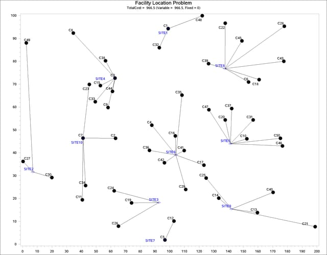
The information printed in the log for the no-fixed-charge model is displayed in Output 7.3.1.
Output 7.3.1: OPTMODEL Log for Facility Location with No Fixed Charges
| NOTE: Problem generation will use 4 threads. |
| NOTE: The problem has 510 variables (0 free, 0 fixed). |
| NOTE: The problem has 510 binary and 0 integer variables. |
| NOTE: The problem has 560 linear constraints (510 LE, 50 EQ, 0 GE, 0 range). |
| NOTE: The problem has 2010 linear constraint coefficients. |
| NOTE: The problem has 0 nonlinear constraints (0 LE, 0 EQ, 0 GE, 0 range). |
| NOTE: The MILP presolver value AUTOMATIC is applied. |
| NOTE: The MILP presolver removed 10 variables and 500 constraints. |
| NOTE: The MILP presolver removed 1010 constraint coefficients. |
| NOTE: The MILP presolver modified 0 constraint coefficients. |
| NOTE: The presolved problem has 500 variables, 60 constraints, and 1000 |
| constraint coefficients. |
| NOTE: The MILP solver is called. |
| Node Active Sols BestInteger BestBound Gap Time |
| 0 1 2 972.1737321 0 972.2 0 |
| 0 1 2 972.1737321 961.2403449 1.14% 0 |
| 0 1 2 972.1737321 966.4828342 0.59% 0 |
| 0 1 3 966.4832160 966.4828342 0.00% 0 |
| NOTE: The MILP solver added 3 cuts with 102 cut coefficients at the root. |
| NOTE: Optimal within relative gap. |
| NOTE: Objective = 966.48321599. |
The results from the warm start approach are shown in Output 7.3.2.
Output 7.3.2: OPTMODEL Log for Facility Location with Fixed Charges, Using Warm Start
| NOTE: Problem generation will use 4 threads. |
| NOTE: The problem has 510 variables (0 free, 0 fixed). |
| NOTE: The problem uses 1 implicit variables. |
| NOTE: The problem has 510 binary and 0 integer variables. |
| NOTE: The problem has 560 linear constraints (510 LE, 50 EQ, 0 GE, 0 range). |
| NOTE: The problem has 2010 linear constraint coefficients. |
| NOTE: The problem has 0 nonlinear constraints (0 LE, 0 EQ, 0 GE, 0 range). |
| NOTE: The MILP presolver value AUTOMATIC is applied. |
| NOTE: The MILP presolver removed 0 variables and 0 constraints. |
| NOTE: The MILP presolver removed 0 constraint coefficients. |
| NOTE: The MILP presolver modified 0 constraint coefficients. |
| NOTE: The presolved problem has 510 variables, 560 constraints, and 2010 |
| constraint coefficients. |
| NOTE: The MILP solver is called. |
| Node Active Sols BestInteger BestBound Gap Time |
| 0 1 3 16070.0150023 0 16070 0 |
| 0 1 3 16070.0150023 9946.2514269 61.57% 0 |
| 0 1 3 16070.0150023 9965.3660728 61.26% 0 |
| 0 1 3 16070.0150023 9992.5098441 60.82% 1 |
| 0 1 3 16070.0150023 10008.1168033 60.57% 1 |
| 0 1 5 12714.8421527 10015.7276884 26.95% 1 |
| 0 1 5 12714.8421527 10022.7765711 26.86% 2 |
| 0 1 6 12697.5037984 10031.4554268 26.58% 2 |
| 0 1 6 12697.5037984 10038.3630945 26.49% 2 |
| 0 1 6 12697.5037984 10040.1836986 26.47% 3 |
| 0 1 7 12681.6662283 10041.2236063 26.30% 3 |
| 0 1 7 12681.6662283 10041.8276236 26.29% 3 |
| 0 1 7 12681.6662283 10042.4192876 26.28% 3 |
| 0 1 7 12681.6662283 10042.4192876 26.28% 6 |
| NOTE: The MILP solver added 30 cuts with 862 cut coefficients at the root. |
| 12 10 10 10982.8321843 10050.5594169 9.28% 7 |
| 113 15 11 10962.4644900 10940.8960590 0.20% 11 |
| 141 16 12 10948.4603467 10942.5795938 0.05% 12 |
| 173 17 13 10948.4603465 10946.1080596 0.02% 12 |
| 181 9 13 10948.4603465 10947.6003284 0.01% 12 |
| NOTE: Optimal within relative gap. |
| NOTE: Objective = 10948.460346. |
The following two SAS programs produce a plot of the solutions for both variants of the model, using data sets produced by PROC OPTMODEL:
title1 h=1.5 "Facility Location Problem";
title2 "TotalCost = &varcostNo (Variable = &varcostNo, Fixed = 0)";

data csdata;
   set cdata(rename=(y=cy)) sdata(rename=(y=sy));
run;

/* create Annotate data set to draw line between customer and assigned site */
%annomac;
data anno(drop=xi yi xj yj);
   %SYSTEM(2, 2, 2);
   set CostNoFixedCharge_Data(keep=xi yi xj yj);
   %LINE(xi, yi, xj, yj, *, 1, 1);
run;

proc gplot data=csdata anno=anno;
   axis1 label=none order=(0 to &xmax by 10);
   axis2 label=none order=(0 to &ymax by 10);
   symbol1 value=dot interpol=none
      pointlabel=("#name" nodropcollisions height=1) cv=black;
   symbol2 value=diamond interpol=none
      pointlabel=("#name" nodropcollisions color=blue height=1) cv=blue;
   plot cy*x sy*x / overlay haxis=axis1 vaxis=axis2;
run;
quit;
The output of the first program is shown in Output 7.3.3.
The output of the second program is shown in Output 7.3.4.
title1 "Facility Location Problem";
title2 "TotalCost = &totalcost (Variable = &varcost, Fixed = &fixcost)";

/* create Annotate data set to draw line between customer and assigned site */
data anno(drop=xi yi xj yj);
   %SYSTEM(2, 2, 2);
   set CostFixedCharge_Data(keep=xi yi xj yj);
   %LINE(xi, yi, xj, yj, *, 1, 1);
run;

proc gplot data=csdata anno=anno;
   axis1 label=none order=(0 to &xmax by 10);
   axis2 label=none order=(0 to &ymax by 10);
   symbol1 value=dot interpol=none
      pointlabel=("#name" nodropcollisions height=1) cv=black;
   symbol2 value=diamond interpol=none
      pointlabel=("#name" nodropcollisions color=blue height=1) cv=blue;
   plot cy*x sy*x / overlay haxis=axis1 vaxis=axis2;
run;
quit;
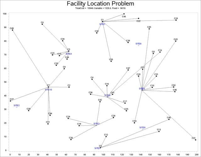
The economic trade-off for the fixed-charge model forces you to build fewer sites and push more demand to each site.
It is possible to expedite the solution of the fixed-charge facility location problem by choosing appropriate branching priorities
for the decision variables. Recall that for each site j, the value of the variable ![]() determines whether or not a facility is built on that site. Suppose you decide to branch on the variables
determines whether or not a facility is built on that site. Suppose you decide to branch on the variables ![]() before the variables
before the variables ![]() . You can set a higher branching priority for
. You can set a higher branching priority for ![]() by using the
by using the .priority suffix for the Build variables in PROC OPTMODEL, as follows:
for{j in SITES} Build[j].priority=10;
Setting higher branching priorities for certain variables is not guaranteed to speed up the MILP solver, but it can be helpful
in some instances. The following program creates and solves an instance of the facility location problem, giving higher priority
to the variables ![]() . The LOGFREQ= option is used to abbreviate the node log.
. The LOGFREQ= option is used to abbreviate the node log.
%let NumCustomers  = 45;
%let NumSites      = 8;
%let SiteCapacity  = 35;
%let MaxDemand     = 10;
%let xmax          = 200;
%let ymax          = 100;
%let seed          = 2345;

/* generate random customer locations */
data cdata(drop=i);
   length name $8;
   do i = 1 to &NumCustomers;
      name = compress('C'||put(i,best.));
      x = ranuni(&seed) * &xmax;
      y = ranuni(&seed) * &ymax;
      demand = ranuni(&seed) * &MaxDemand;
      output;
   end;
run;

/* generate random site locations and fixed charge */
data sdata(drop=i);
length name $8;
   do i = 1 to &NumSites;
      name = compress('SITE'||put(i,best.));
      x = ranuni(&seed) * &xmax;
      y = ranuni(&seed) * &ymax;
      fixed_charge = (abs(&xmax/2-x) + abs(&ymax/2-y)) / 2;
      output;
   end;
run;
proc optmodel;
   set <str> CUSTOMERS;
   set <str> SITES init {};

   /* x and y coordinates of CUSTOMERS and SITES */
   num x {CUSTOMERS union SITES};
   num y {CUSTOMERS union SITES};
   num demand {CUSTOMERS};
   num fixed_charge {SITES};

   /* distance from customer i to site j */
   num dist {i in CUSTOMERS, j in SITES}
       = sqrt((x[i] - x[j])^2 + (y[i] - y[j])^2);

   read data cdata into CUSTOMERS=[name] x y demand;
   read data sdata into SITES=[name] x y fixed_charge;

   var Assign {CUSTOMERS, SITES} binary;
   var Build {SITES} binary;

   min CostFixedCharge
       = sum {i in CUSTOMERS, j in SITES} dist[i,j] * Assign[i,j]
         + sum {j in SITES} fixed_charge[j] * Build[j];

   /* each customer assigned to exactly one site */
   con assign_def {i in CUSTOMERS}:
      sum {j in SITES} Assign[i,j] = 1;

   /* if customer i assigned to site j, then facility must be built at j */
   con link {i in CUSTOMERS, j in SITES}:
      Assign[i,j] <= Build[j];

   /* each site can handle at most &SiteCapacity demand */
   con capacity {j in SITES}:
      sum {i in CUSTOMERS} demand[i] * Assign[i,j] <= &SiteCapacity * Build[j];

   /* assign priority to Build variables (y) */
   for{j in SITES} Build[j].priority=10;

   /* solve the MILP with fixed charges, using branching priorities */
   solve obj CostFixedCharge with milp / logfreq=1000;
quit;
The resulting output is shown in Output 7.3.5.
Output 7.3.5: PROC OPTMODEL Log for Facility Location with Branching Priorities
| NOTE: There were 45 observations read from the data set WORK.CDATA. |
| NOTE: There were 8 observations read from the data set WORK.SDATA. |
| NOTE: Problem generation will use 4 threads. |
| NOTE: The problem has 368 variables (0 free, 0 fixed). |
| NOTE: The problem has 368 binary and 0 integer variables. |
| NOTE: The problem has 413 linear constraints (368 LE, 45 EQ, 0 GE, 0 range). |
| NOTE: The problem has 1448 linear constraint coefficients. |
| NOTE: The problem has 0 nonlinear constraints (0 LE, 0 EQ, 0 GE, 0 range). |
| NOTE: The MILP presolver value AUTOMATIC is applied. |
| NOTE: The MILP presolver removed 0 variables and 0 constraints. |
| NOTE: The MILP presolver removed 0 constraint coefficients. |
| NOTE: The MILP presolver modified 0 constraint coefficients. |
| NOTE: The presolved problem has 368 variables, 413 constraints, and 1448 |
| constraint coefficients. |
| NOTE: The MILP solver is called. |
| Node Active Sols BestInteger BestBound Gap Time |
| 0 1 3 2823.1827978 0 2823.2 0 |
| 0 1 3 2823.1827978 1727.0208789 63.47% 0 |
| 0 1 3 2823.1827978 1752.0649013 61.13% 0 |
| 0 1 3 2823.1827978 1764.4145721 60.01% 0 |
| 0 1 3 2823.1827978 1771.3542742 59.38% 1 |
| 0 1 3 2823.1827978 1778.1649446 58.77% 1 |
| 0 1 3 2823.1827978 1779.9319639 58.61% 1 |
| 0 1 3 2823.1827978 1780.4398220 58.57% 1 |
| 0 1 6 1903.7976887 1781.4348074 6.87% 2 |
| 0 1 6 1903.7976887 1781.6818875 6.85% 2 |
| 0 1 6 1903.7976887 1781.9825516 6.84% 2 |
| 0 1 6 1903.7976887 1784.3735066 6.69% 2 |
| 0 1 6 1903.7976887 1785.1171912 6.65% 3 |
| 0 1 6 1903.7976887 1785.1318270 6.65% 3 |
| 0 1 6 1903.7976887 1785.1691077 6.65% 3 |
| 0 1 6 1903.7976887 1785.2000207 6.64% 3 |
| 0 1 6 1903.7976887 1785.2000207 6.64% 3 |
| NOTE: The MILP solver added 28 cuts with 767 cut coefficients at the root. |
| 4 1 8 1852.5588919 1802.5216297 2.78% 4 |
| 52 46 10 1835.0251598 1804.8458565 1.67% 5 |
| 244 215 11 1834.9126635 1808.0082480 1.49% 7 |
| 296 245 12 1830.7850312 1809.1809114 1.19% 8 |
| 523 282 13 1825.1666003 1812.4410890 0.70% 11 |
| 608 293 14 1825.1666001 1814.3493473 0.60% 13 |
| 642 135 15 1821.5115363 1815.4351037 0.33% 13 |
| 691 46 16 1819.9124342 1818.1426710 0.10% 13 |
| 735 4 16 1819.9124342 1819.7466770 0.01% 14 |
| NOTE: Optimal within relative gap. |
| NOTE: Objective = 1819.9124342. |