The Linear Programming Solver

Example 5.5 Using the Network Simplex Solver

This example demonstrates how you can use the network simplex solver to find the minimum-cost flow in a directed graph. Consider the directed graph in Figure 5.4, which appears in Ahuja, Magnanti, and Orlin (1993).

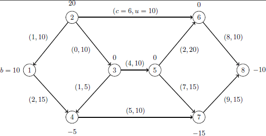
Figure 5.4 Minimum Cost Network Flow Problem: Data

You can use the following SAS statements to create the input data sets nodedata and arcdata:

data nodedata;
   input _node_ $ _sd_;
   datalines;
1    10
2    20
3     0
4    -5
5     0
6     0
7   -15
8   -10
;
run;

data arcdata;
   input _tail_ $ _head_ $ _lo_ _capac_ _cost_;
   datalines;
1    4    0    15    2
2    1    0    10    1
2    3    0    10    0
2    6    0    10    6
3    4    0     5    1
3    5    0    10    4
4    7    0    10    5
5    6    0    20    2
5    7    0    15    7 
6    8    0    10    8
7    8    0    15    9
;
run;

You can use the following call to PROC OPTMODEL to find the minimum-cost flow:

proc optmodel;
   set <str> NODES;
   num supply_demand {NODES};

   set <str,str> ARCS;
   num arcLower  {ARCS};
   num arcUpper  {ARCS};
   num arcCost   {ARCS};

   read data arcdata into ARCS=[_tail_ _head_] 
      arcLower=_lo_ arcUpper=_capac_ arcCost=_cost_;
   read data nodedata into NODES=[_node_] supply_demand=_sd_;

   var flow {<i,j> in ARCS} >= arcLower[i,j] <= arcUpper[i,j];
   min obj = sum {<i,j> in ARCS} arcCost[i,j] * flow[i,j];
   con balance {i in NODES}:
      sum {<(i),j> in ARCS} flow[i,j] - sum {<j,(i)> in ARCS} flow[j,i] 
         = supply_demand[i]; 
   solve with lp / solver=ns scale=none printfreq=1;
   print flow;
quit;
%put &_OROPTMODEL_;

The optimal solution is displayed in Output 5.5.1.

Output 5.5.1 Network Simplex Solver: Primal Solution Output

The OPTMODEL Procedure

Problem Summary
Objective Sense	Minimization
Objective Function	obj
Objective Type	Linear

Number of Variables	11
Bounded Above	0
Bounded Below	0
Bounded Below and Above	11
Free	0
Fixed	0

Number of Constraints	8
Linear LE (<=)	0
Linear EQ (=)	8
Linear GE (>=)	0
Linear Range	0

Constraint Coefficients	22

Solution Summary
Solver	Network Simplex
Objective Function	obj
Solution Status	Optimal
Objective Value	270
Iterations	8
Iterations2	1

Primal Infeasibility	0
Dual Infeasibility	0
Bound Infeasibility	0

[1]	[2]	flow
1	4	10
2	1	0
2	3	10
2	6	10
3	4	5
3	5	5
4	7	10
5	6	0
5	7	5
6	8	10
7	8	0

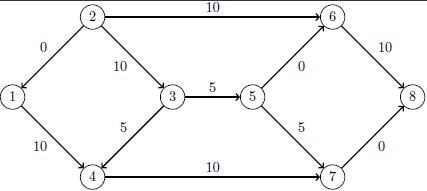
The optimal solution is represented graphically in Figure 5.5.

Figure 5.5 Minimum Cost Network Flow Problem: Optimal Solution

The iteration log is displayed in Output 5.5.2.

Output 5.5.2 Log: Solution Progress

NOTE: There were 11 observations read from the data set WORK.ARCDATA.

NOTE: There were 8 observations read from the data set WORK.NODEDATA.

NOTE: The problem has 11 variables (0 free, 0 fixed).

NOTE: The problem has 8 linear constraints (0 LE, 8 EQ, 0 GE, 0 range).

NOTE: The problem has 22 linear constraint coefficients.

NOTE: The problem has 0 nonlinear constraints (0 LE, 0 EQ, 0 GE, 0 range).

NOTE: The PRESOLVER value NONE is applied because a pure network has been found.

NOTE: The OPTLP presolver value NONE is applied.

NOTE: The NETWORK SIMPLEX solver is called.

NOTE: The network has 8 rows (100.00%), 11 columns (100.00%), and 1 component.

NOTE: The network extraction and setup time is 0.00 seconds.

Iteration PrimalObj PrimalInf Time

1 0 20.0000000 0.00

2 0 20.0000000 0.00

3 5.0000000 15.0000000 0.00

4 5.0000000 15.0000000 0.00

5 75.0000000 15.0000000 0.00

6 75.0000000 15.0000000 0.00

7 130.0000000 10.0000000 0.00

8 270.0000000 0 0.00

NOTE: The Network Simplex solve time is 0.00 seconds.

NOTE: The total Network Simplex solve time is 0.00 seconds.

NOTE: Optimal.

NOTE: Objective = 270.

NOTE: The PRIMAL SIMPLEX solver is called.

Objective Entering Leaving

Phase Iteration Value Variable Variable

2 1 270.000000 flow['2','1'] flow['4','7'](S)

NOTE: Optimal.

NOTE: Objective = 270.

STATUS=OK SOLUTION_STATUS=OPTIMAL OBJECTIVE=270 PRIMAL_INFEASIBILITY=0

DUAL_INFEASIBILITY=0 BOUND_INFEASIBILITY=0 ITERATIONS=8 ITERATIONS2=1

PRESOLVE_TIME=0.00 SOLUTION_TIME=0.00

Now, suppose there is a budget on the flow that comes out of arc 2: the total arc cost of flow that comes out of arc 2 cannot exceed 50. You can use the following call to PROC OPTMODEL to find the minimum-cost flow:

proc optmodel;
   set <str> NODES;
   num supply_demand {NODES};

   set <str,str> ARCS;
   num arcLower  {ARCS};
   num arcUpper  {ARCS};
   num arcCost   {ARCS};

   read data arcdata into ARCS=[_tail_ _head_] 
      arcLower=_lo_ arcUpper=_capac_ arcCost=_cost_;
   read data nodedata into NODES=[_node_] supply_demand=_sd_;

   var flow {<i,j> in ARCS} >= arcLower[i,j] <= arcUpper[i,j];
   min obj = sum {<i,j> in ARCS} arcCost[i,j] * flow[i,j];
   con balance {i in NODES}:
      sum {<(i),j> in ARCS} flow[i,j] - sum {<j,(i)> in ARCS} flow[j,i] 
         = supply_demand[i]; 
   con budgetOn2:
      sum {<i,j> in ARCS: i='2'} arcCost[i,j] * flow[i,j] <= 50;
   solve with lp / solver=ns scale=none printfreq=1;
   print flow;
quit;
%put &_OROPTMODEL_;

The optimal solution is displayed in Output 5.5.3.

Output 5.5.3 Network Simplex Solver: Primal Solution Output

The OPTMODEL Procedure

Problem Summary
Objective Sense	Minimization
Objective Function	obj
Objective Type	Linear

Number of Variables	11
Bounded Above	0
Bounded Below	0
Bounded Below and Above	11
Free	0
Fixed	0

Number of Constraints	9
Linear LE (<=)	1
Linear EQ (=)	8
Linear GE (>=)	0
Linear Range	0

Constraint Coefficients	24

Solution Summary
Solver	Network Simplex
Objective Function	obj
Solution Status	Optimal
Objective Value	274
Iterations	5
Iterations2	2

Primal Infeasibility	8.881784E-16
Dual Infeasibility	0
Bound Infeasibility	0

[1]	[2]	flow
1	4	12
2	1	2
2	3	10
2	6	8
3	4	3
3	5	7
4	7	10
5	6	2
5	7	5
6	8	10
7	8	0

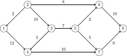
The optimal solution is represented graphically in Figure 5.6.

Figure 5.6 Minimum Cost Network Flow Problem: Optimal Solution (with Budget Constraint)

The iteration log is displayed in Output 5.5.4. Note that the network simplex solver extracts a subnetwork in this case.

Output 5.5.4 Log: Solution Progress

NOTE: There were 11 observations read from the data set WORK.ARCDATA.

NOTE: There were 8 observations read from the data set WORK.NODEDATA.

NOTE: The problem has 11 variables (0 free, 0 fixed).

NOTE: The problem has 9 linear constraints (1 LE, 8 EQ, 0 GE, 0 range).

NOTE: The problem has 24 linear constraint coefficients.

NOTE: The problem has 0 nonlinear constraints (0 LE, 0 EQ, 0 GE, 0 range).

NOTE: The OPTLP presolver value AUTOMATIC is applied.

NOTE: The OPTLP presolver removed 6 variables and 7 constraints.

NOTE: The OPTLP presolver removed 15 constraint coefficients.

NOTE: The presolved problem has 5 variables, 2 constraints, and 9 constraint

coefficients.

NOTE: The NETWORK SIMPLEX solver is called.

NOTE: The network has 1 rows (50.00%), 5 columns (100.00%), and 1 component.

NOTE: The network extraction and setup time is 0.00 seconds.

Iteration PrimalObj PrimalInf Time

1 259.9800000 5.0200000 0.00

2 264.9900000 0.0100000 0.00

3 265.0300000 0 0.00

4 255.0300000 0 0.00

5 270.0000000 0 0.00

NOTE: The Network Simplex solve time is 0.00 seconds.

NOTE: The total Network Simplex solve time is 0.00 seconds.

NOTE: Optimal.

NOTE: Objective = 270.

NOTE: The DUAL SIMPLEX solver is called.

Objective Entering Leaving

Phase Iteration Value Variable Variable

2 1 270.000000 flow['5','6'] budgetOn2 (S)

2 2 274.000000 flow['3','4'] flow['2','3'](S)

NOTE: Optimal.

NOTE: Objective = 274.

STATUS=OK SOLUTION_STATUS=OPTIMAL OBJECTIVE=274

PRIMAL_INFEASIBILITY=8.881784E-16 DUAL_INFEASIBILITY=0 BOUND_INFEASIBILITY=0

ITERATIONS=5 ITERATIONS2=2 PRESOLVE_TIME=0.00 SOLUTION_TIME=0.00