The Sequential Quadratic Programming Solver: Choosing a Good Starting Point :: SAS/OR(R) 9.22 User's Guide: Mathematical Programming

The Sequential Quadratic Programming Solver

Example 15.3 Choosing a Good Starting Point

To solve a constrained nonlinear optimization problem, both the optimal primal and optimal dual variables have to be computed. Therefore, a good estimate of both the primal and dual variables is essential for fast convergence. An important feature of the SQP solver is that it computes a good estimate of the dual variables if an estimate of the primal variables is known.

The following example illustrates how a good initial starting point helps in securing the desired optimum:

$\text{[math]}$

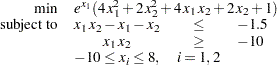Assume the starting point $\text{[math]}$ = (30, –30). The SAS code is as follows:

proc optmodel;
   var x {1..2} <= 8 >= -10;   /* variable bounds */
       
   minimize obj = 
      exp(x[1])*(4*x[1]^2 + 2*x[2]^2 + 4*x[1]*x[2] + 2*x[2] + 1);
   
   con consl: 
      x[1]*x[2] -x[1] - x[2] <= -1.5;
   con cons2:
      x[1]*x[2] >= -10;
   
   x[1] = 30; x[2] = -30; /* starting point */
   solve with sqp / printfreq = 5 ;
   print x;

The solution (a local optimum) obtained by the SQP solver is displayed in Output 15.3.1.

Output 15.3.1 Solution Obtained with the Starting Point (30, –30)

The OPTMODEL Procedure

Problem Summary
Objective Sense	Minimization
Objective Function	obj
Objective Type	Nonlinear

Number of Variables	2
Bounded Above	0
Bounded Below	0
Bounded Below and Above	2
Free	0
Fixed	0

Number of Constraints	2
Linear LE (<=)	0
Linear EQ (=)	0
Linear GE (>=)	0
Linear Range	0
Nonlinear LE (<=)	1
Nonlinear EQ (=)	0
Nonlinear GE (>=)	1
Nonlinear Range	0

Solution Summary
Solver	SQP
Objective Function	obj
Solution Status	Optimal
Objective Value	0.0235503931
Iterations	32

Infeasibility	0
Optimality Error	3.5739607E-6
Complementarity	4.0620922E-7

[1]	x
1	-9.5474
2	1.0474

You can find a solution with a smaller objective value by assuming a starting point of (–10, 1). Continue to submit the following code:

   
   /* starting point */
   x[1] = -10;
   x[2] =  1;
   
   solve with sqp / printfreq = 5 ;
   print x;
   quit;

The corresponding solution is displayed in Output 15.3.2.

Output 15.3.2 Solution Obtained with the Starting Point (–10, 1)

The OPTMODEL Procedure

Problem Summary
Objective Sense	Minimization
Objective Function	obj
Objective Type	Nonlinear

Number of Variables	2
Bounded Above	0
Bounded Below	0
Bounded Below and Above	2
Free	0
Fixed	0

Number of Constraints	2
Linear LE (<=)	0
Linear EQ (=)	0
Linear GE (>=)	0
Linear Range	0
Nonlinear LE (<=)	1
Nonlinear EQ (=)	0
Nonlinear GE (>=)	1
Nonlinear Range	0

Solution Summary
Solver	SQP
Objective Function	obj
Solution Status	Optimal
Objective Value	0.0235504281
Iterations	10

Infeasibility	0
Optimality Error	8.8391537E-7
Complementarity	1.444755E-6

[1]	x
1	-9.5474
2	1.0474

The preceding illustration demonstrates the importance of a good starting point in obtaining the optimal solution. The SQP solver ensures global convergence only to a local optimum. Therefore you need to have sufficient knowledge of your problem in order to be able to get a "good" estimate of the starting point.

Top of Page