| The Sequential Quadratic Programming Solver |
| Conditions of Optimality |
To facilitate discussion of the optimality conditions, we present the notation to be used for easy reference:

number of general nonlinear constraints, which include the linear constraints but not the bound constraints

dimension of
 , i.e., the number of decision variables
 iterate, i.e., the vector of
decision variables 
objective function

gradient of the objective function

Hessian matrix of the objective function

Lagrange multiplier vector,


Lagrangian function of constrained problems

gradient of the Lagrangian function with respect to
For and , the superscript  is used to denote the value at the th iteration, such as
  , and the superscript
  is used to denote their corresponding optimal values, such as
  .
.
We rewrite the general form of nonlinear optimization problems in the section Overview: SQP Solver by grouping the equality constraints and inequality constraints. We also rewrite all the general nonlinear inequality constraints and bound constraints in one form as " " inequality constraints. Thus we have the following:
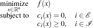 |
where  is the set of indices of the equality constraints,
  is the set of indices of the inequality constraints, and
  .
.
A point is feasible if it satisfies all the constraints  , and
, and  . The feasible region
  consists of all the feasible points. In unconstrained cases, the feasible region is the entire
  space.
A feasible point  is a local solution of the problem if there exists a neighborhood
  of such that
 |
Further, a feasible point is a strict local solution if strict inequality holds in the preceding case, i.e.,
 |
A feasible point is a global solution of the problem if no point in has a smaller function value than  ), i.e.,
 |
The SQP solver finds a local minimum of an optimization problem.
Unconstrained Optimization
The following conditions hold for unconstrained optimization problems:
First-order necessary conditions: If
is a local solution and is continuously differentiable in some neighborhood of , then 
Second-order necessary conditions: If
is a local solution and is twice continuously differentiable in some neighborhood of , then  is positive semidefinite.
 Second-order sufficient conditions: If
is twice continuously differentiable in some neighborhood of , and if  and is positive definite, then is a strict local solution.
Constrained Optimization
For constrained optimization problems, the Lagrangian function is defined as follows:
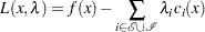 |
where  , are called Lagrange multipliers. is used to denote the gradient of the Lagrangian function with respect to , and
  is used to denote the Hessian of the Lagrangian function with respect to . The active set at a feasible point is defined as
 |
We also need the following definition before we can state the first-order and second-order necessary conditions:
Linear independence constraint qualification and regular point: A point
is said to satisfy the linear independence constraint qualification if the gradients of active constraints 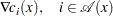
are linearly independent. We refer to such a point
as a regular point.
We now state the theorems that are essential in the analysis and design of algorithms for constrained optimization:
First-order necessary conditions: Suppose
is a local minimum and also a regular point. If and  , are continuously differentiable, there exist Lagrange multipliers
  such that the following conditions hold:
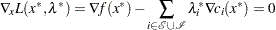
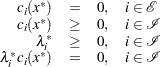
The preceding conditions are often known as the Karush-Kuhn-Tucker conditions, or KKT conditions for short.
Second-order necessary conditions: Suppose
is a local minimum and also a regular point. Let be the Lagrange multipliers that satisfy the KKT conditions. If and  , are twice continuously differentiable, the following conditions hold:
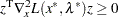
for all
 that satisfy
Second-order sufficient conditions: Suppose there exist a point
and some Lagrange multipliers such that the KKT conditions are satisfied. If the conditions 
hold for all
 that satisfy
 then
is a strict local solution. Note that the set of all such
 ’s forms the null space of matrix
  . Hence we can numerically check the Hessian of the Lagrangian function projected onto the null space. For a rigorous treatment of the optimality conditions, see Fletcher (1987) and Nocedal and Wright (1999).
Solver’s Criteria
The SQP solver declares a solution to be optimal when all the following criteria are satisfied:
The relative norm of the gradient of the Lagrangian function is less than OPTTOL, and the absolute norm of the gradient of the Lagrangian function is less than 1.0E–2.
When the problem is a constrained optimization problem, the relative norm of the gradient of the Lagrangian function is defined as

When the problem is an unconstrained optimization problem, it is defined as

The absolute value of each equality constraint is less than FEASTOL.
The value of each "
 " inequality is greater than the right-hand-side constant minus FEASTOL.
 The value of each "
 " inequality is less than the right-hand-side constant plus FEASTOL.
 The value of each Lagrange multiplier for inequalities is greater than
 OPTTOL.
 The minimum of both the values of an inequality and its corresponding Lagrange multiplier is less than OPTTOL.
The last four points imply that the complementarity error, defined as  ,
,  , approaches zero as the solver progresses.
The SQP solver provides the HESCHECK option to verify that the second-order necessary conditions are also satisfied.
Copyright © SAS Institute, Inc. All Rights Reserved.