| The Quadratic Programming Solver |
Example 14.1 Linear Least Squares Problem
The linear least squares problem arises in the context of determining a solution to an over-determined set of linear equations. In practice, these could arise in data fitting and estimation problems. An over-determined system of linear equations can be defined as
 |
where  ,
,  ,
,  , and
, and  . Since this system usually does not have a solution, we need to be satisfied with some sort of approximate solution. The most widely used approximation is the least squares solution, which minimizes
  .
.
This problem is called a least squares problem for the following reason. Let  ,
,  , and
, and  be defined as previously. Let
  be the
  th component of the vector
  :
:
 |
By definition of the Euclidean norm, the objective function can be expressed as follows:
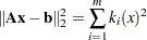 |
Therefore the function we minimize is the sum of squares of  terms ; hence the term least squares. The following example is an illustration of the linear least squares problem; i.e., each of the terms
  is a linear function of
  .
.
Consider the following least squares problem defined by
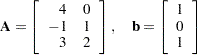 |
This translates to the following set of linear equations:
 |
The corresponding least squares problem is
 |
The preceding objective function can be expanded to
 |
In addition, we impose the following constraint so that the equation  is satisfied within a tolerance of
  :
:
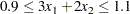 |
You can use the following SAS code to solve the least squares problem:
/* example 1: linear least-squares problem */
proc optmodel;
   var x1; /* declare free (no explicit bounds) variable x1 */
   var x2; /* declare free (no explicit bounds) variable x2 */
   /* declare slack variable for ranged constraint */
   var w >= 0 <= 0.2;

   /* objective function: minimize is the sum of squares */
   minimize f = 26 * x1 * x1 + 5 * x2 * x2 + 10 * x1 * x2
       - 14 * x1 - 4 * x2 + 2;

   /* subject to the following constraint */
   con L: 3 * x1 + 2 * x2 - w = 0.9;

   solve with qp;

   /* print the optimal solution */
   print x1 x2;
quit;
The output is shown in Output 14.1.1.
| Problem Summary | |
|---|---|
| Objective Sense | Minimization |
| Objective Function | f |
| Objective Type | Quadratic |
| Number of Variables | 3 |
| Bounded Above | 0 |
| Bounded Below | 0 |
| Bounded Below and Above | 1 |
| Free | 2 |
| Fixed | 0 |
| Number of Constraints | 1 |
| Linear LE (<=) | 0 |
| Linear EQ (=) | 1 |
| Linear GE (>=) | 0 |
| Linear Range | 0 |
Note: This procedure is experimental.
Copyright © SAS Institute, Inc. All Rights Reserved.