PROC OPTMODEL: Model Construction :: SAS/OR(R) 9.22 User's Guide: Mathematical Programming

The OPTMODEL Procedure

Example 8.3 Model Construction

This example uses PROC OPTMODEL features to simplify the construction of a mathematically formulated model. The model is based on the section An Assignment Problem in the PROC LP documentation. A single invocation of PROC OPTMODEL replaces several steps in the PROC LP code.

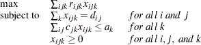
The model assigns production of various grades of cloth to a set of machines in order to maximize profit while meeting customer demand. Each machine has different capacities to produce the various grades of cloth. (See the PROC LP example for more details.) The mathematical formulation, where $\text{[math]}$ represents the amount of cloth of grade $\text{[math]}$ to produce on machine $\text{[math]}$ for customer $\text{[math]}$ , follows:

$\text{[math]}$

The following code defines the same data sets used in the PROC LP example to specify the problem coefficients:

title 'An Assignment Problem'; 

data object; 
   input machine customer 
         grade1 grade2 grade3 grade4 grade5 grade6; 
   datalines; 
1 1 102 140 105  105  125  148 
1 2 115 133 118  118  143  166 
1 3  70 108  83   83   88   86 
1 4  79 117  87   87  107  105 
1 5  77 115  90   90  105  148 
2 1 123 150 125  124  154   . 
2 2 130 157 132  131  166   . 
2 3 103 130 115  114  129   . 
2 4 101 128 108  107  137   . 
2 5 118 145 130  129  154   . 
3 1  83  .   .    97  122  147 
3 2 119  .   .   133  163  180 
3 3  67  .   .    91  101  101 
3 4  85  .   .   104  129  129 
3 5  90  .   .   114  134  179 
4 1 108 121  79   .   112  132 
4 2 121 132  92   .   130  150 
4 3  78  91  59   .    77   72 
4 4 100 113  76   .   109  104 
4 5  96 109  77   .   105  145 
;

data demand; 
   input customer 
         grade1 grade2 grade3 grade4 grade5 grade6; 
   datalines; 
1 100 100 150  150  175  250 
2 300 125 300  275  310  325 
3 400   0 400  500  340    0 
4 250   0 750  750    0    0 
5   0 600 300    0  210  360 
;

data resource; 
   input machine 
         grade1 grade2 grade3 grade4 grade5 grade6 avail; 
   datalines; 
1 .250 .275 .300  .350  .310  .295  744 
2 .300 .300 .305  .315  .320  .     244 
3 .350 .    .     .320  .315  .300  790 
4 .280 .275 .260  .     .250  .295  672 
;

The following PROC OPTMODEL code specifies the model, processes the input data sets, solves the optimization problem, and generates a solution data set:

proc optmodel;
   set CUSTOMERS;
   set GRADES = 1..6;
   set MACHINES;
   /* parameters */
   number return{CUSTOMERS, GRADES, MACHINES} init 0;
   number demand{CUSTOMERS, GRADES};
   number cost{GRADES,MACHINES} init 0;
   number avail{MACHINES} init 0;
   /* load the customer set and demands */
   read data demand
        into CUSTOMERS=[customer]
        {j in GRADES} <demand[customer,j]=col("grade"||j)>;
   /* load the machine set, time costs, and availability */
   read data resource nomiss
        into MACHINES=[machine] 
        {j in GRADES} <cost[j,machine]=col("grade"||j)>
        avail;
   /* load objective data */
   read data object nomiss
        into [machine customer]
        {j in GRADES} <return[customer,j,machine]=col("grade"||j)>;
   /* the model */
   var x{CUSTOMERS, GRADES, MACHINES} >= 0;
   max obj = sum{i in CUSTOMERS, j in GRADES, k in MACHINES}
             return[i,j,k] * x[i,j,k];
   con req_demand{i in CUSTOMERS, j in GRADES}:
       sum{k in MACHINES} x[i,j,k] = demand[i,j];
   con req_avail{k in MACHINES}:
       sum{i in CUSTOMERS, j in GRADES} 
          cost[j,k]*x[i,j,k] <= avail[k];
   /* fix x[i,j,k] to 0 if cost[j,k] = 0 */
   for {j in GRADES, k in MACHINES: cost[j,k] = 0} do;
      for {i in CUSTOMERS} fix x[i,j,k]=0;
   end;
   
   /* call the solver and save the results */
   solve with lp/solver=primal;
   create data solution 
          from [customer grade machine]
          ={i in CUSTOMERS, j in GRADES,k in MACHINES: x[i,j,k] NE 0}
          amount=x;
   quit;

PROC OPTMODEL processes the data sets directly, using the READ DATA statements to load the data into suitably declared numeric parameters. The READ DATA statements use the iterated column syntax to transfer a range of data set variables into indexed parameters. The COL name expression is expanded in each case into the input data set variables grade1 to grade6. Missing values in the input data sets are handled by using the NOMISS option and initializing the parameters to zero.

For simplicity, the preceding code assumes a fixed set of cloth grades. However, the number of grades could be read from another data set or determined by using SAS functions to examine the variables in the data sets. The first and second READ DATA statements assign the customer and machine sets, respectively, with the set of index values read from the input data sets.

The model portion of the PROC OPTMODEL code parallels the mathematical formulation of the linear program. The solver produces the following output:

Output 8.3.1 LP Solver Result

An Assignment Problem

Problem Summary
Objective Sense	Maximization
Objective Function	obj
Objective Type	Linear

Number of Variables	120
Bounded Above	0
Bounded Below	100
Bounded Below and Above	0
Free	0
Fixed	20

Number of Constraints	34
Linear LE (<=)	4
Linear EQ (=)	30
Linear GE (>=)	0
Linear Range	0

Solution Summary
Solver	Primal Simplex
Objective Function	obj
Solution Status	Optimal
Objective Value	871426.03763
Iterations	37

Primal Infeasibility	0
Dual Infeasibility	0
Bound Infeasibility	0

The CREATE DATA statement writes the solution variables to a data set after the solver finishes executing. The explicit source index set is used to restrict the output to the nonzero solution variables. This data set can be processed by PROC TABULATE as follows to create a compact representation of the solution:

proc tabulate data=solution; 
   class customer grade machine; 
   var   amount; 
   table (machine*customer), (grade*amount); 
run;

This code produces the table shown in Output 8.3.2.

Output 8.3.2 An Assignment Problem

An Assignment Problem

		grade
		1	2	3	4	5	6
		amount	amount	amount	amount	amount	amount
		Sum	Sum	Sum	Sum	Sum	Sum
machine	customer	.	100.00	150.00	150.00	175.00	250.00
1	1	.	100.00	150.00	150.00	175.00	250.00
	2	.	.	300.00	.	.	.
	3	.	.	256.72	210.31	.	.
	4	.	.	750.00	.	.	.
	5	.	92.27	.	.	.	.
2	3	.	.	143.28	.	340.00	.
2	5	.	.	300.00	.	.	.
3	2	.	.	.	275.00	310.00	325.00
	3	.	.	.	289.69	.	.
	4	.	.	.	750.00	.	.
	5	.	.	.	.	210.00	360.00
4	1	100.00	.	.	.	.	.
	2	300.00	125.00	.	.	.	.
	3	400.00	.	.	.	.	.
	4	250.00	.	.	.	.	.
	5	.	507.73	.	.	.	.

Top of Page