Previous Page | Next Page

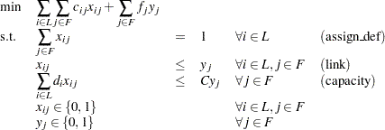
The OPTMILP Procedure

Example 18.3 Facility Location

This advanced example demonstrates how to warm start PROC OPTMILP by using the PRIMALIN= option. The model is constructed in PROC OPTMODEL and saved in an MPS-format SAS data set for use in PROC OPTMILP. Note that this problem can also be solved from within PROC OPTMODEL; see Chapter 11 for details.

Consider the classical facility location problem. Given a set of customer locations and a set of candidate facility sites, you must decide which sites to build facilities on and assign coverage of customer demand to these sites so as to minimize cost. All customer demand must be satisfied, and each facility has a demand capacity limit . The total cost is the sum of the distances between facility and its assigned customer , plus a fixed charge for building a facility at site . Let represent choosing site to build a facility, and 0 otherwise. Also, let represent the assignment of customer to facility , and 0 otherwise. This model can be formulated as the following integer linear program:


Constraint (assign_def) ensures that each customer is assigned to exactly one site. Constraint (link) forces a facility to be built if any customer has been assigned to that facility. Finally, constraint (capacity) enforces the capacity limit at each site.

Let us also consider a variation of this same problem where there is no cost for building a facility. This problem is typically easier to solve than the original problem. For this variant, let the objective be


First, let us construct a random instance of this problem by using the following DATA steps:

                                                                                                         
   %let NumCustomers  = 50; 
   %let NumSites      = 10; 
   %let SiteCapacity  = 35; 
   %let MaxDemand     = 10; 
   %let xmax          = 200;
   %let ymax          = 100;  
   %let seed          = 938; 
                                                                                                                                        
   /* generate random customer locations */                                                                                             
   data cdata(drop=i);                                                                                                                  
      length name $8;                                                                                                                   
      do i = 1 to &NumCustomers;                                                                                                        
         name = compress('C'||put(i,best.));                                                                                            
         x = ranuni(&seed) * &xmax;                                                                                                     
         y = ranuni(&seed) * &ymax;                                                                                                     
         demand = ranuni(&seed) * &MaxDemand;                                                                                           
         output;                                                                                                                        
      end;                                                                                                                              
   run;                                                                                                                                 
                                                                                                                                        
   /* generate random site locations and fixed charge */                                                                                
   data sdata(drop=i);                                                                                                                  
      length name $8;                                                                                                                   
      do i = 1 to &NumSites;                                                                                                            
         name = compress('SITE'||put(i,best.));                                                                                         
         x = ranuni(&seed) * &xmax;                                                                                                     
         y = ranuni(&seed) * &ymax;                                                                                                     
         fixed_charge = 30 * (abs(&xmax/2-x) + abs(&ymax/2-y));                                                                      
         output;                                                                                                                        
      end;                                                                                                                              
   run;                                                                                                                                 

In the following PROC OPTMODEL code, we generate the model and define both variants of the cost function:

                                                                                                       
proc optmodel;                                                                                                                      
   set <str> CUSTOMERS;                                                                                                              
   set <str> SITES init {};                                                                                                                  
                                                                                                                                     
   /* x and y coordinates of CUSTOMERS and SITES */                                                                                  
   num x {CUSTOMERS union SITES};                                                                                                    
   num y {CUSTOMERS union SITES};                                                                                                    
   num demand {CUSTOMERS};                                                                                                            
   num fixed_charge {SITES};                                                                                                         
                                                                                                                                     
   /* distance from customer i to site j */                                                                                          
   num dist {i in CUSTOMERS, j in SITES}                                                                                             
       = sqrt((x[i] - x[j])^2 + (y[i] - y[j])^2);                                                                                    
                                                                                                                                     
   read data cdata into CUSTOMERS=[name] x y demand;                                                                                 
   read data sdata into SITES=[name] x y fixed_charge;                                                                               
                                                                                                                                     
   var Assign {CUSTOMERS, SITES} binary;                                                                                             
   var Build {SITES} binary;                                                                                                             
   /* each customer assigned to exactly one site */                                                                                  
   con assign_def {i in CUSTOMERS}:                                                                                                  
       sum {j in SITES} Assign[i,j] = 1;                                                                                              
                                                                                                                                     
   /* if customer i assigned to site j, then facility must be */
   /* built at j                                              */                                                          
   con link {i in CUSTOMERS, j in SITES}:                                                                                            
       Assign[i,j] <= Build[j];                                                                                                      
                                                                                                                                     
   /* each site can handle at most &SiteCapacity demand */                                                                           
   con capacity {j in SITES}:                                                                                                        
       sum {i in CUSTOMERS} demand[i] * Assign[i,j] 
       <= &SiteCapacity * Build[j];                                                     
                                                                                                                                                                  
   min CostNoFixedCharge                                                                                                             
       = sum {i in CUSTOMERS, j in SITES} dist[i,j] * Assign[i,j]; 
       
   save mps nofcdata;
   min CostFixedCharge                                                                                                               
       = CostNoFixedCharge 
         + sum {j in SITES} fixed_charge[j] * Build[j]; 
       
   save mps fcdata;
   
quit;    

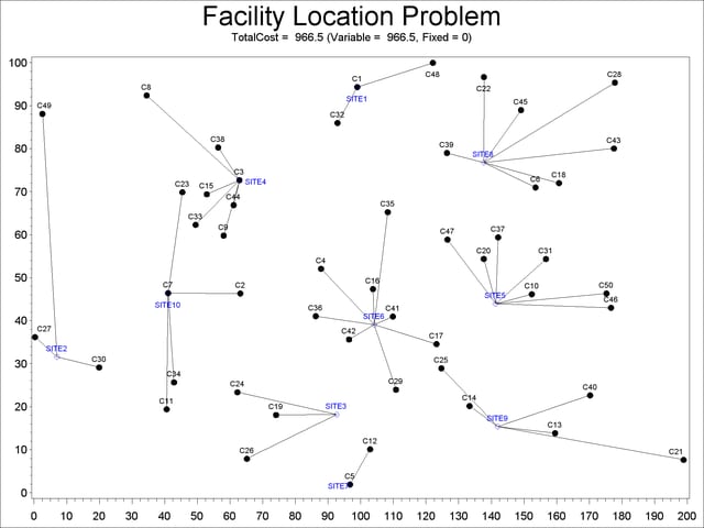
We first solve the problem for the model with no fixed charge by using the following code. The first PROC SQL call populates the macro variables varcostNo. This macro variable is used to display the objective value when the results are plotted. The second PROC SQL call generates a data set which is used to plot the results. The information printed in the log by PROC OPTMILP is displayed in Output 18.3.1.

proc optmilp data=nofcdata primalout=nofcout;
run;

proc sql noprint;
   select put(sum(_objcoef_ * _value_),6.1) into :varcostNo
   from nofcout;
quit;

proc sql;
   create table CostNoFixedCharge_Data as
   select
      scan(p._var_,2,'[],') as customer,
      scan(p._var_,3,'[],') as site,
      c.x as xi, c.y as yi, s.x as xj, s.y as yj
   from
      cdata as c, 
      sdata as s, 
      nofcout(where=(substr(_var_,1,6)='Assign' and 
                     round(_value_) = 1)) as p
   where calculated customer = c.name and calculated site = s.name;
quit;

Output 18.3.1 PROC OPTMILP Log for Facility Location with No Fixed Charges


NOTE: The problem nofcdata has 510 variables (510 binary, 0 integer, 0 free, 0   
      fixed).                                                                    
NOTE: The problem has 560 constraints (510 LE, 50 EQ, 0 GE, 0 range).            
NOTE: The problem has 2010 constraint coefficients.                              
NOTE: The OPTMILP presolver value AUTOMATIC is applied.                          
NOTE: The OPTMILP presolver removed 10 variables and 500 constraints.            
NOTE: The OPTMILP presolver removed 1010 constraint coefficients.                
NOTE: The OPTMILP presolver modified 0 constraint coefficients.                  
NOTE: The presolved problem has 500 variables, 60 constraints, and 1000          
      constraint coefficients.                                                   
NOTE: The MIXED INTEGER LINEAR solver is called.                                 
          Node  Active    Sols    BestInteger      BestBound      Gap    Time    
             0       1       0              .    961.2403449        .       0    
             0       1       2    966.4832160    966.4832160    0.00%       0    
             0       0       2    966.4832160              .    0.00%       0    
NOTE: OPTMILP added 3 cuts with 172 cut coefficients at the root.                
NOTE: Optimal.                                                                   
NOTE: Objective = 966.483216.                                                    
NOTE: The data set WORK.NOFCOUT has 510 observations and 8 variables.            


Next, we solve the fixed-charge model by using the following code. Note that the solution to the model with no fixed charge is feasible for the fixed-charge model and should provide a good starting point for PROC OPTMILP. We use the PRIMALIN= option to provide an incumbent solution ("warm start"). The two PROC SQL calls perform the same functions as in the case with no fixed charges. The results from this approach are shown in Output 18.3.2.

proc optmilp data=fcdata primalin=nofcout;
run;

proc sql noprint;
   select put(sum(_objcoef_ * _value_), 6.1) into :varcost
   from fcout(where=(substr(_var_,1,6)='Assign'));
   select put(sum(_objcoef_ * _value_), 5.1) into :fixcost
   from fcout(where=(substr(_var_,1,5)='Build'));
   select put(sum(_objcoef_ * _value_), 6.1) into :totalcost
   from fcout;
quit;
   
proc sql;
   create table CostFixedCharge_Data as
   select
      scan(p._var_,2,'[],') as customer,
      scan(p._var_,3,'[],') as site,
      c.x as xi, c.y as yi, s.x as xj, s.y as yj
   from
      cdata as c, 
      sdata as s, 
      fcout(where=(substr(_var_,1,6)='Assign' and 
                   round(_value_) = 1)) as p
   where calculated customer = c.name and calculated site = s.name;
quit;

Output 18.3.2 PROC OPTMILP Log for Facility Location with Fixed Charges, Using Warm Start


NOTE: The problem fcdata has 510 variables (510 binary, 0 integer, 0 free, 0     
      fixed).                                                                    
NOTE: The problem has 560 constraints (510 LE, 50 EQ, 0 GE, 0 range).            
NOTE: The problem has 2010 constraint coefficients.                              
NOTE: The OPTMILP presolver value AUTOMATIC is applied.                          
NOTE: The OPTMILP presolver removed 0 variables and 0 constraints.               
NOTE: The OPTMILP presolver removed 0 constraint coefficients.                   
NOTE: The OPTMILP presolver modified 0 constraint coefficients.                  
NOTE: The presolved problem has 510 variables, 560 constraints, and 2010         
      constraint coefficients.                                                   
NOTE: The MIXED INTEGER LINEAR solver is called.                                 
          Node  Active    Sols    BestInteger      BestBound      Gap    Time    
             0       1       1  18157.3952518   9946.2514269   82.56%       0    
             0       1       1  18157.3952518  10927.3069327   66.17%       0    
             0       1       3  12709.9206825  10939.4930100   16.18%       0    
             0       1       3  12709.9206825  10940.9262264   16.17%       0    
             0       1       3  12709.9206825  10941.3574623   16.16%       0    
             0       1       5  10972.1286676  10943.6017601    0.26%       0    
             0       1       5  10972.1286676  10944.4165350    0.25%       0    
             0       1       6  10958.2477272  10944.9725321    0.12%       0    
             0       1       7  10953.4634076  10944.9749576    0.08%       0    
             0       1       7  10953.4634076  10945.0677477    0.08%       0    
             0       1       7  10953.4634076  10945.0698887    0.08%       0    
             0       1       7  10953.4634076  10945.0981211    0.08%       0    
NOTE: OPTMILP added 20 cuts with 2249 cut coefficients at the root.              
            17       8       8  10950.3308516  10945.4549713    0.04%       1    
            19       9       9  10950.3308490  10945.4549713    0.04%       1    
            24       8      10  10950.0345546  10946.0684050    0.04%       1    
            26      10      11  10949.9022613  10946.0684050    0.04%       1    
            35       0      12  10948.4603416              .    0.00%       1    
NOTE: Optimal.                                                                   
NOTE: Objective = 10948.4603.                                                    
NOTE: The data set WORK.FCOUT has 510 observations and 8 variables.              


The following two SAS programs produce a plot of the solutions for both variants of the model, using data sets produced by PROC SQL from the PRIMALOUT= data sets produced by PROC OPTMILP.

Note:Execution of this code requires SAS/GRAPH software.

                                                                                                       
title1 "Facility Location Problem";  
title2 "TotalCost = &varcostNo (Variable = &varcostNo, Fixed = 0)";
data csdata;                                                                                                                        
   set cdata(rename=(y=cy)) sdata(rename=(y=sy));                                                                                  
run;                                                                                                                                
/* create Annotate data set to draw line between customer and */
/* assigned site                                              */                                                      
%annomac;                                                                                                                           
data anno(drop=xi yi xj yj);                                                                                                        
   %SYSTEM(2, 2, 2);                                                                                                                
set CostNoFixedCharge_Data(keep=xi yi xj yj);                                                                                    
   %LINE(xi, yi, xj, yj, *, 1, 1);                                                                                                  
run;   
proc gplot data=csdata anno=anno;                                                                                                   
   axis1 label=none order=(0 to &xmax by 10);                                                                                       
   axis2 label=none order=(0 to &ymax by 10);                                                                                       
   symbol1 value=dot interpol=none                                                                                                                                                                    
      pointlabel=("#name" nodropcollisions height=0.7) cv=black;                                                                  
   symbol2 value=diamond interpol=none                                                                                                                                                      
      pointlabel=("#name" nodropcollisions color=blue height=0.7) cv=blue;                                                                   
   plot cy*x sy*x / overlay haxis=axis1 vaxis=axis2;                                                                                
run;
quit;   

The output from the first program appears in Output 18.3.3.

Output 18.3.3 Solution Plot for Facility Location with No Fixed Charges
Solution Plot for Facility Location with No Fixed Charges

                                                                                                      
title1 "Facility Location Problem";  
title2 "TotalCost = &totalcost (Variable = &varcost, Fixed = &fixcost)";
/* create Annotate data set to draw line between customer and */
/* assigned site                                              */                                                      
data anno(drop=xi yi xj yj);                                                                                                        
   %SYSTEM(2, 2, 2);                                                                                                               
   set CostFixedCharge_Data(keep=xi yi xj yj);                                                                                      
   %LINE(xi, yi, xj, yj, *, 1, 1);                                                                                                  
run;  
proc gplot data=csdata anno=anno;                                                                                                   
   axis1 label=none order=(0 to &xmax by 10);                                                                                       
   axis2 label=none order=(0 to &ymax by 10);                                                                                       
   symbol1 value=dot interpol=none                                                                                                                                                                  
      pointlabel=("#name" nodropcollisions height=0.7) cv=black;                                                                    
   symbol2 value=diamond interpol=none                                                                                                                                                     
      pointlabel=("#name" nodropcollisions color=blue height=0.7) cv=blue;                                                                    
   plot cy*x sy*x / overlay haxis=axis1 vaxis=axis2;                                                                                
run;
quit;   

The output from the second program appears in Output 18.3.4.

Output 18.3.4 Solution Plot for Facility Location with Fixed Charges
Solution Plot for Facility Location with Fixed Charges

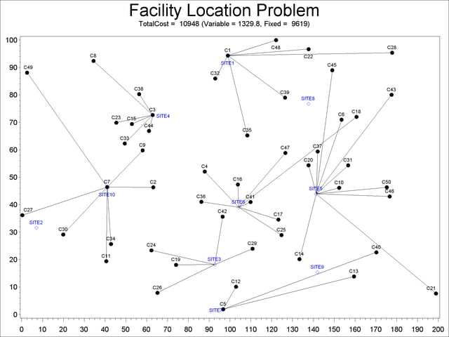
The economic tradeoff for the fixed-charge model forces us to build fewer sites and push more demand to each site.

Previous Page | Next Page | Top of Page