The Mixed Integer Linear Programming Solver: Facility Location :: SAS/OR(R) 9.22 User's Guide: Mathematical Programming

The Mixed Integer Linear Programming Solver

Example 11.3 Facility Location

Consider the classic facility location problem. Given a set $\text{[math]}$ of customer locations and a set $\text{[math]}$ of candidate facility sites, you must decide which sites to build facilities on and assign coverage of customer demand to these sites so as to minimize cost. All customer demand $\text{[math]}$ must be satisfied, and each facility has a demand capacity limit $\text{[math]}$ . The total cost is the sum of the distances $\text{[math]}$ between facility $\text{[math]}$ and its assigned customer $\text{[math]}$ , plus a fixed charge $\text{[math]}$ for building a facility at site $\text{[math]}$ . Let $\text{[math]}$ represent choosing site $\text{[math]}$ to build a facility, and 0 otherwise. Also, let $\text{[math]}$ represent the assignment of customer $\text{[math]}$ to facility $\text{[math]}$ , and 0 otherwise. This model can be formulated as the following integer linear program:

$\text{[math]}$

Constraint (assign_def) ensures that each customer is assigned to exactly one site. Constraint (link) forces a facility to be built if any customer has been assigned to that facility. Finally, constraint (capacity) enforces the capacity limit at each site.

Let us also consider a variation of this same problem where there is no cost for building a facility. This problem is typically easier to solve than the original problem. For this variant, let the objective be

$\text{[math]}$

First, let us construct a random instance of this problem by using the following DATA steps:

                                                                                                         
   %let NumCustomers  = 50;
   %let NumSites      = 10; 
   %let SiteCapacity  = 35;
   %let MaxDemand     = 10; 
   %let xmax          = 200;
   %let ymax          = 100; 
   %let seed          = 938; 
                                                                                                                                        
   /* generate random customer locations */                                                                                             
   data cdata(drop=i);                                                                                                                  
      length name $8;                                                                                                                   
      do i = 1 to &NumCustomers;                                                                                                        
         name = compress('C'||put(i,best.));                                                                                            
         x = ranuni(&seed) * &xmax;                                                                                                     
         y = ranuni(&seed) * &ymax;                                                                                                     
         demand = ranuni(&seed) * &MaxDemand;                                                                                           
         output;                                                                                                                        
      end;                                                                                                                              
   run;                                                                                                                                 
                                                                                                                                        
   /* generate random site locations and fixed charge */                                                                                
   data sdata(drop=i);                                                                                                                  
      length name $8;                                                                                                                   
      do i = 1 to &NumSites;                                                                                                            
         name = compress('SITE'||put(i,best.));                                                                                         
         x = ranuni(&seed) * &xmax;                                                                                                     
         y = ranuni(&seed) * &ymax;                                                                                                     
         fixed_charge = 30 * (abs(&xmax/2-x) + abs(&ymax/2-y));                                                                
         output;                                                                                                                        
      end;                                                                                                                              
   run;

In the following PROC OPTMODEL code, we first generate and solve the model with the no-fixed-charge variant of the cost function. Next, we solve the fixed-charge model. Note that the solution to the model with no fixed charge is feasible for the fixed-charge model and should provide a good starting point for the MILP solver. We use the PRIMALIN option to provide an incumbent solution (warm start).

                                                                                                       

proc optmodel;
    set <str> CUSTOMERS;
    set <str> SITES init {};
    
    /* x and y coordinates of CUSTOMERS and SITES */
    num x {CUSTOMERS union SITES};
    num y {CUSTOMERS union SITES};
    num demand {CUSTOMERS};
    num fixed_charge {SITES};
    
    /* distance from customer i to site j */
    num dist {i in CUSTOMERS, j in SITES}
        = sqrt((x[i] - x[j])^2 + (y[i] - y[j])^2);
    
    read data cdata into CUSTOMERS=[name] x y demand;
    read data sdata into SITES=[name] x y fixed_charge;
    
    var Assign {CUSTOMERS, SITES} binary;
    var Build {SITES} binary;
    
    min CostNoFixedCharge
        = sum {i in CUSTOMERS, j in SITES} dist[i,j] * Assign[i,j];
    min CostFixedCharge
        = CostNoFixedCharge + sum {j in SITES} fixed_charge[j] * Build[j];
    
    /* each customer assigned to exactly one site */
    con assign_def {i in CUSTOMERS}:
       sum {j in SITES} Assign[i,j] = 1;
    
    /* if customer i assigned to site j, then facility must be built at j */
    con link {i in CUSTOMERS, j in SITES}:
        Assign[i,j] <= Build[j];
    
    /* each site can handle at most &SiteCapacity demand */
    con capacity {j in SITES}:
        sum {i in CUSTOMERS} demand[i] * Assign[i,j] <= 
            &SiteCapacity * Build[j];
    
    /* solve the MILP with no fixed charges */      
    solve obj CostNoFixedCharge with milp / printfreq = 500;      
    
    /* clean up the solution */
    for {i in CUSTOMERS, j in SITES} Assign[i,j] = round(Assign[i,j]);
    for {j in SITES} Build[j] = round(Build[j]);
    
    call symput('varcostNo',put(CostNoFixedCharge,6.1));
    
    /* create a data set for use by GPLOT */
    create data CostNoFixedCharge_Data from
        [customer site]={i in CUSTOMERS, j in SITES: Assign[i,j] = 1}
        xi=x[i] yi=y[i] xj=x[j] yj=y[j];
    
    /* solve the MILP, with fixed charges with warm start */
    solve obj CostFixedCharge with milp / primalin printfreq = 500;
    
    /* clean up the solution */
    for {i in CUSTOMERS, j in SITES} Assign[i,j] = round(Assign[i,j]);
    for {j in SITES} Build[j] = round(Build[j]);
    
    num varcost = sum {i in CUSTOMERS, j in SITES} dist[i,j] * Assign[i,j].sol;
    num fixcost = sum {j in SITES} fixed_charge[j] * Build[j].sol;
    call symput('varcost', put(varcost,6.1));
    call symput('fixcost', put(fixcost,5.1));
    call symput('totalcost', put(CostFixedCharge,6.1));
    
    /* create a data set for use by GPLOT */
    create data CostFixedCharge_Data from
        [customer site]={i in CUSTOMERS, j in SITES: Assign[i,j] = 1}
        xi=x[i] yi=y[i] xj=x[j] yj=y[j];
 quit;

The information printed in the log for the no-fixed-charge model is displayed in Output 11.3.1.

Output 11.3.1 OPTMODEL Log for Facility Location with No Fixed Charges


NOTE: The problem has 510 variables (0 free, 0 fixed).
NOTE: The problem has 510 binary and 0 integer variables.
NOTE: The problem has 560 linear constraints (510 LE, 50 EQ, 0 GE, 0 range).
NOTE: The problem has 2010 linear constraint coefficients.
NOTE: The problem has 0 nonlinear constraints (0 LE, 0 EQ, 0 GE, 0 range).
NOTE: The OPTMODEL presolver removed 0 variables, 0 linear constraints, and 0
nonlinear constraints.
NOTE: The OPTMILP presolver value AUTOMATIC is applied.
NOTE: The OPTMILP presolver removed 10 variables and 500 constraints.
NOTE: The OPTMILP presolver removed 1010 constraint coefficients.
NOTE: The OPTMILP presolver modified 0 constraint coefficients.
NOTE: The presolved problem has 500 variables, 60 constraints, and 1000
constraint coefficients.
NOTE: The MIXED INTEGER LINEAR solver is called.
Node Active Sols BestInteger BestBound Gap Time
0 1 0 . 961.2403449 . 0
0 1 2 966.4832160 966.4832160 0.00% 0
0 0 2 966.4832160 . 0.00% 0
NOTE: OPTMILP added 3 cuts with 172 cut coefficients at the root.
NOTE: Optimal.
NOTE: Objective = 966.483216.

The results from the warm start approach are shown in Output 11.3.2.

Output 11.3.2 OPTMODEL Log for Facility Location with Fixed Charges, Using Warm Start


NOTE: The problem has 510 variables (0 free, 0 fixed).
NOTE: The problem uses 1 implicit variables.
NOTE: The problem has 510 binary and 0 integer variables.
NOTE: The problem has 560 linear constraints (510 LE, 50 EQ, 0 GE, 0 range).
NOTE: The problem has 2010 linear constraint coefficients.
NOTE: The problem has 0 nonlinear constraints (0 LE, 0 EQ, 0 GE, 0 range).
NOTE: The OPTMODEL presolver removed 0 variables, 0 linear constraints, and 0
nonlinear constraints.
NOTE: The OPTMILP presolver value AUTOMATIC is applied.
NOTE: The OPTMILP presolver removed 0 variables and 0 constraints.
NOTE: The OPTMILP presolver removed 0 constraint coefficients.
NOTE: The OPTMILP presolver modified 0 constraint coefficients.
NOTE: The presolved problem has 510 variables, 560 constraints, and 2010
constraint coefficients.
NOTE: The MIXED INTEGER LINEAR solver is called.
Node Active Sols BestInteger BestBound Gap Time
0 1 1 18157.3952518 9946.2514269 82.56% 0
0 1 1 18157.3952518 10928.0104852 66.15% 0
0 1 1 18157.3952518 10936.9480810 66.02% 0
0 1 1 18157.3952518 10940.8705927 65.96% 0
0 1 3 10972.1286676 10941.8588583 0.28% 0
0 1 3 10972.1286676 10942.0276578 0.28% 0
0 1 3 10972.1286676 10943.1109102 0.27% 0
0 1 4 10950.3308631 10943.4163218 0.06% 0
0 1 4 10950.3308631 10943.5610209 0.06% 0
0 1 4 10950.3308631 10944.0007474 0.06% 0
0 1 4 10950.3308631 10944.1330756 0.06% 0
0 1 4 10950.3308631 10944.3631088 0.05% 0
NOTE: OPTMILP added 18 cuts with 2011 cut coefficients at the root.
6 7 5 10948.4603327 10944.5884206 0.04% 0
14 0 5 10948.4603327 . 0.00% 0
NOTE: Optimal.
NOTE: Objective = 10948.4603.

The following two SAS programs produce a plot of the solutions for both variants of the model, using data sets produced by PROC OPTMODEL.

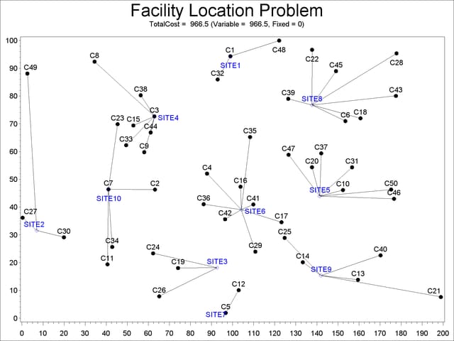
title1 "Facility Location Problem";                                                                                                 
title2 "TotalCost = &varcostNo (Variable = &varcostNo, Fixed = 0)";                                                               
data csdata;                                                                                                                        
    set cdata(rename=(y=cy)) sdata(rename=(y=sy));                                                                                  
run;                                                                                                                                
/* create Annotate data set to draw line between customer and assigned site */                                                      
%annomac;                                                                                                                           
data anno(drop=xi yi xj yj);                                                                                                        
   %SYSTEM(2, 2, 2);                                                                                                               
   set CostNoFixedCharge_Data(keep=xi yi xj yj);                                                                                    
   %LINE(xi, yi, xj, yj, *, 1, 1);                                                                                                  
run;
proc gplot data=csdata anno=anno;                                                                                                   
   axis1 label=none order=(0 to &xmax by 10);                                                                                       
   axis2 label=none order=(0 to &ymax by 10);                                                                                       
   symbol1 value=dot interpol=none                                                                                                  
      pointlabel=("#name" nodropcollisions height=1) cv=black;                                                                   
   symbol2 value=diamond interpol=none                                                                                              
      pointlabel=("#name" nodropcollisions color=blue height=1) cv=blue;                                                                    
   plot cy*x sy*x / overlay haxis=axis1 vaxis=axis2;                                                                                
run;
quit;

The output of the first program is shown in Output 11.3.3.

Output 11.3.3 Solution Plot for Facility Location with No Fixed Charges

The output of the second program is shown in Output 11.3.4.

title1 "Facility Location Problem";                                                                                                 
title2 "TotalCost = &totalcost (Variable = &varcost, Fixed = &fixcost)";                                                        
/* create Annotate data set to draw line between customer and assigned site */                                                      
data anno(drop=xi yi xj yj);                                                                                                        
   %SYSTEM(2, 2, 2);                                                                                                                
   set CostFixedCharge_Data(keep=xi yi xj yj);                                                                                      
   %LINE(xi, yi, xj, yj, *, 1, 1);                                                                                                  
run;
proc gplot data=csdata anno=anno;                                                                                                   
   axis1 label=none order=(0 to &xmax by 10);                                                                                       
   axis2 label=none order=(0 to &ymax by 10);                                                                                       
   symbol1 value=dot interpol=none                                                                                                  
      pointlabel=("#name" nodropcollisions height=1) cv=black;                                                                    
   symbol2 value=diamond interpol=none                                                                                              
      pointlabel=("#name" nodropcollisions color=blue height=1) cv=blue;                                                                    
   plot cy*x sy*x / overlay haxis=axis1 vaxis=axis2;                                                                                
run;
quit;

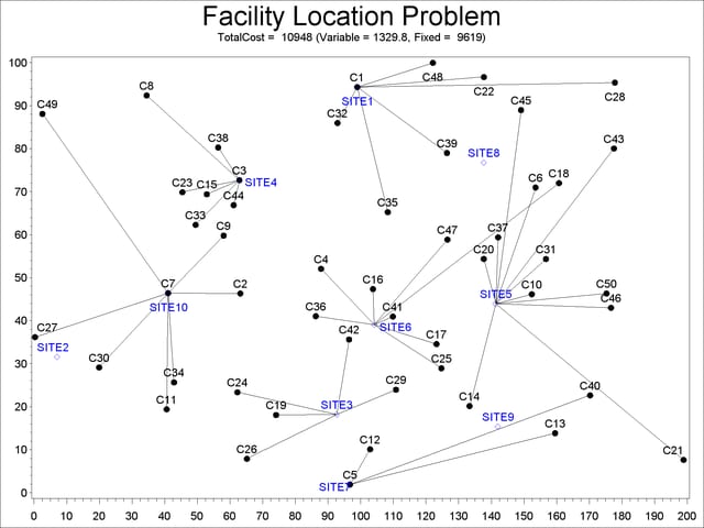
Output 11.3.4 Solution Plot for Facility Location with Fixed Charges

The economic trade-off for the fixed-charge model forces us to build fewer sites and push more demand to each site.

It is possible to expedite the solution of the fixed-charge facility location problem by choosing appropriate branching priorities for the decision variables. Recall that for each site $\text{[math]}$ , the value of the variable $\text{[math]}$ determines whether or not a facility is built on that site. Suppose you decide to branch on the variables $\text{[math]}$ before the variables $\text{[math]}$ . You can set a higher branching priority for $\text{[math]}$ by using the .priority suffix for the Build variables in PROC OPTMODEL, as follows:

for{j in SITES} Build[j].priority=10;

Setting higher branching priorities for certain variables is not guaranteed to speed up the MILP solver, but it can be helpful in some instances. The following program creates and solves an instance of the facility location problem in which giving higher priority to $\text{[math]}$ causes the MILP solver to find the optimal solution more quickly. We use the PRINTFREQ= option to abbreviate the node log.

   
    %let NumCustomers  = 45;    
    %let NumSites      = 8;    
    %let SiteCapacity  = 35;    
    %let MaxDemand     = 10;    
    %let xmax          = 200;    
    %let ymax          = 100;    
    %let seed          = 2345;

    /* generate random customer locations */
    data cdata(drop=i);
       length name $8;
       do i = 1 to &NumCustomers;
          name = compress('C'||put(i,best.));
          x = ranuni(&seed) * &xmax;
          y = ranuni(&seed) * &ymax;
          demand = ranuni(&seed) * &MaxDemand;
          output;
       end;
    run;

    /* generate random site locations and fixed charge */
    data sdata(drop=i);
       length name $8;
       do i = 1 to &NumSites;
          name = compress('SITE'||put(i,best.));
          x = ranuni(&seed) * &xmax;
          y = ranuni(&seed) * &ymax;
          fixed_charge = (abs(&xmax/2-x) + abs(&ymax/2-y)) / 2;
          output;
       end;
    run;

proc optmodel;                                                                                                                                                                                                                        
   set <str> CUSTOMERS;
   set <str> SITES init {};
   /* x and y coordinates of CUSTOMERS and SITES */
   num x {CUSTOMERS union SITES};
   num y {CUSTOMERS union SITES};
   num demand {CUSTOMERS};
   num fixed_charge {SITES};
       
   /* distance from customer i to site j */
   num dist {i in CUSTOMERS, j in SITES} 
       = sqrt((x[i] - x[j])^2 + (y[i] - y[j])^2);
   read data cdata into CUSTOMERS=[name] x y demand;
   read data sdata into SITES=[name] x y fixed_charge;
   var Assign {CUSTOMERS, SITES} binary;
   var Build {SITES} binary;
   min CostFixedCharge   
       = sum {i in CUSTOMERS, j in SITES} dist[i,j] * Assign[i,j] 
         + sum {j in SITES} fixed_charge[j] * Build[j];
   
   /* each customer assigned to exactly one site */
   con assign_def {i in CUSTOMERS}:
      sum {j in SITES} Assign[i,j] = 1;
   /* if customer i assigned to site j, then facility must be built at j */
   con link {i in CUSTOMERS, j in SITES}:
       Assign[i,j] <= Build[j];
   /* each site can handle at most &SiteCapacity demand */
   con capacity {j in SITES}:
       sum {i in CUSTOMERS} demand[i] * Assign[i,j] <= &SiteCapacity * Build[j];
   /* assign priority to Build variables (y) */
   for{j in SITES} Build[j].priority=10;
   /* solve the MILP with fixed charges, using branching priorities */
   solve obj CostFixedCharge with milp / printfreq=1000;
   
quit;

The resulting output is shown in Output 11.3.5.

Output 11.3.5 PROC OPTMODEL Log for Facility Location with Branching Priorities

Facility Location Problem

TotalCost = 10948 (Variable = 1329.8, Fixed = 9619)


NOTE: There were 45 observations read from the data set WORK.CDATA.
NOTE: There were 8 observations read from the data set WORK.SDATA.
NOTE: The problem has 368 variables (0 free, 0 fixed).
NOTE: The problem has 368 binary and 0 integer variables.
NOTE: The problem has 413 linear constraints (368 LE, 45 EQ, 0 GE, 0 range).
NOTE: The problem has 1448 linear constraint coefficients.
NOTE: The problem has 0 nonlinear constraints (0 LE, 0 EQ, 0 GE, 0 range).
NOTE: The OPTMODEL presolver removed 0 variables, 0 linear constraints, and 0
nonlinear constraints.
NOTE: The OPTMILP presolver value AUTOMATIC is applied.
NOTE: The OPTMILP presolver removed 0 variables and 0 constraints.
NOTE: The OPTMILP presolver removed 0 constraint coefficients.
NOTE: The OPTMILP presolver modified 0 constraint coefficients.
NOTE: The presolved problem has 368 variables, 413 constraints, and 1448
constraint coefficients.
NOTE: The MIXED INTEGER LINEAR solver is called.
Node Active Sols BestInteger BestBound Gap Time
0 1 0 . 1727.0208789 . 0
0 1 0 . 1752.4772119 . 0
0 1 0 . 1766.8871214 . 0
0 1 0 . 1782.4679173 . 0
0 1 0 . 1789.7457043 . 0
0 1 0 . 1795.4885663 . 0
0 1 0 . 1796.5823017 . 0
0 1 0 . 1797.6560556 . 0
0 1 0 . 1798.7536497 . 0
0 1 2 1913.6380522 1800.4984668 6.28% 0
0 1 2 1913.6380522 1801.6361692 6.22% 0
0 1 2 1913.6380522 1802.1482666 6.19% 0
0 1 3 1837.6796606 1802.2534725 1.97% 0
0 1 3 1837.6796606 1802.2775684 1.96% 0
0 1 3 1837.6796606 1802.2882515 1.96% 0
0 1 3 1837.6796606 1802.2968289 1.96% 0
NOTE: OPTMILP added 31 cuts with 1325 cut coefficients at the root.
417 377 4 1837.3598299 1807.9546113 1.63% 1
493 301 6 1827.4464378 1808.3524685 1.06% 1
618 369 7 1827.2477982 1809.7356078 0.97% 2
651 188 8 1819.9124343 1809.9044615 0.55% 2
661 197 9 1819.9124343 1809.9044615 0.55% 2
904 6 9 1819.9124343 1819.7809841 0.01% 2
NOTE: Optimal within relative gap.
NOTE: Objective = 1819.91243.

The output in Output 11.3.6 is generated by running the same program without the line that assigns higher branching priorities to the Build variables. We again use the PRINTFREQ= option to abbreviate the node log.

proc optmodel;                                                                                                                                                                                                                         
   set <str> CUSTOMERS;
   set <str> SITES init {};
   /* x and y coordinates of CUSTOMERS and SITES */
   num x {CUSTOMERS union SITES};
   num y {CUSTOMERS union SITES};
   num demand {CUSTOMERS};
   num fixed_charge {SITES};
       
   /* distance from customer i to site j */
   num dist {i in CUSTOMERS, j in SITES} 
       = sqrt((x[i] - x[j])^2 + (y[i] - y[j])^2);
   read data cdata into CUSTOMERS=[name] x y demand;
   read data sdata into SITES=[name] x y fixed_charge;
   var Assign {CUSTOMERS, SITES} binary;
   var Build {SITES} binary;
   min CostFixedCharge   
       = sum {i in CUSTOMERS, j in SITES} dist[i,j] * Assign[i,j] 
         + sum {j in SITES} fixed_charge[j] * Build[j];
   
   /* each customer assigned to exactly one site */
   con assign_def {i in CUSTOMERS}:
      sum {j in SITES} Assign[i,j] = 1;
   /* if customer i assigned to site j, then facility must be built at j */
   con link {i in CUSTOMERS, j in SITES}:
       Assign[i,j] <= Build[j];
   /* each site can handle at most &SiteCapacity demand */
   con capacity {j in SITES}:
       sum {i in CUSTOMERS} demand[i] * Assign[i,j] <= &SiteCapacity * Build[j];
       
   /* solve the MILP with fixed charges, using branching priorities */
   solve obj CostFixedCharge with milp / printfreq=10000;
   
quit;

Output 11.3.6 PROC OPTMODEL Log for Facility Location without Branching Priorities

Facility Location Problem

TotalCost = 10948 (Variable = 1329.8, Fixed = 9619)


NOTE: There were 45 observations read from the data set WORK.CDATA.
NOTE: There were 8 observations read from the data set WORK.SDATA.
NOTE: The problem has 368 variables (0 free, 0 fixed).
NOTE: The problem has 368 binary and 0 integer variables.
NOTE: The problem has 413 linear constraints (368 LE, 45 EQ, 0 GE, 0 range).
NOTE: The problem has 1448 linear constraint coefficients.
NOTE: The problem has 0 nonlinear constraints (0 LE, 0 EQ, 0 GE, 0 range).
NOTE: The OPTMODEL presolver removed 0 variables, 0 linear constraints, and 0
nonlinear constraints.
NOTE: The OPTMILP presolver value AUTOMATIC is applied.
NOTE: The OPTMILP presolver removed 0 variables and 0 constraints.
NOTE: The OPTMILP presolver removed 0 constraint coefficients.
NOTE: The OPTMILP presolver modified 0 constraint coefficients.
NOTE: The presolved problem has 368 variables, 413 constraints, and 1448
constraint coefficients.
NOTE: The MIXED INTEGER LINEAR solver is called.
Node Active Sols BestInteger BestBound Gap Time
0 1 0 . 1727.0208789 . 0
0 1 0 . 1752.4772119 . 0
0 1 0 . 1766.8871214 . 0
0 1 0 . 1782.4679173 . 0
0 1 0 . 1789.7457043 . 0
0 1 0 . 1795.4885663 . 0
0 1 0 . 1796.5823017 . 0
0 1 0 . 1797.6560556 . 0
0 1 0 . 1798.7536497 . 0
0 1 2 1913.6380522 1800.4984668 6.28% 0
0 1 2 1913.6380522 1801.6361692 6.22% 0
0 1 2 1913.6380522 1802.1482666 6.19% 0
0 1 3 1837.6796606 1802.2534725 1.97% 0
0 1 3 1837.6796606 1802.2775684 1.96% 0
0 1 3 1837.6796606 1802.2882515 1.96% 0
0 1 3 1837.6796606 1802.2968289 1.96% 0
NOTE: OPTMILP added 31 cuts with 1325 cut coefficients at the root.
417 377 4 1837.3598299 1807.9546113 1.63% 1
493 301 6 1827.4464378 1808.3524685 1.06% 1
618 369 7 1827.2477982 1809.7356078 0.97% 2
651 188 8 1819.9124343 1809.9044615 0.55% 2
661 197 9 1819.9124343 1809.9044615 0.55% 2
904 6 9 1819.9124343 1819.7809841 0.01% 2
NOTE: Optimal within relative gap.
NOTE: Objective = 1819.91243.

By comparing Output 11.3.5 and Output 11.3.6 you can see that in this instance, increasing the branching priorities of the Build variables results in computational savings.

Top of Page