The Interior Point NLP Solver

Getting Started: IPNLP Solver

The IPNLP solver consists of two techniques that can solve a wide class of optimization problems efficiently and robustly. In this section two examples that introduce the two techniques of IPNLP are presented. The examples also introduce basic features of the modeling language of PROC OPTMODEL that is used to define the optimization problem.

The IPNLP solver can be invoked using the SOLVE statement:

SOLVE WITH IPNLP </ options> ;

where options specify the technique name, termination criteria, and how to display the results in the iteration log. For a detailed description of the options, see the section IPNLP Solver Options.

A Simple Problem

Consider the following simple example of a nonlinear optimization problem:

$\text{[math]}$

The problem consists of a quadratic objective function, a linear equality, and a nonlinear inequality constraint. You want to find a local minimum, starting from the point 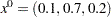$\text{[math]}$ . To achieve this, you write the following statements:

proc optmodel;
   var x{1..3} >= 0;
   minimize obj = ( x[1] + 3*x[2] + x[3] )**2 + 4*(x[1] - x[2])**2;

   con constr1: sum{i in 1..3}x[i] = 1;
   con constr2: 6*x[2] + 4*x[3] - x[1]**3 -3 >= 0;

   /* starting point */
   x[1] = 0.1;
   x[2] = 0.7;
   x[3] = 0.2;

   solve with IPNLP;
   print x;
quit;

Note that there is no option specified. Therefore, the default solver is used to solve the problem. The SAS output displays a detailed summary of the problem, together with the status of the solver at termination, the total number of iterations required, and the value of the objective function at the local minimum. The summary and the optimal solution are shown in Output 9.1.

Figure 9.1 Problem Summary and the Optimal Solution

The OPTMODEL Procedure

Problem Summary
Objective Sense	Minimization
Objective Function	obj
Objective Type	Quadratic

Number of Variables	3
Bounded Above	0
Bounded Below	3
Bounded Below and Above	0
Free	0
Fixed	0

Number of Constraints	2
Linear LE (<=)	0
Linear EQ (=)	1
Linear GE (>=)	0
Linear Range	0
Nonlinear LE (<=)	0
Nonlinear EQ (=)	0
Nonlinear GE (>=)	1
Nonlinear Range	0

Solution Summary
Solver	IPNLP/IPQN
Objective Function	obj
Solution Status	Optimal
Objective Value	1.0000053879
Iterations	21

Infeasibility	2.810568E-10
Optimality Error	7.8706805E-7

[1]	x
1	0.00071696
2	0.00000083
3	0.99928221

The SAS log shown in Output 9.2 displays a brief summary of the problem being solved, followed by the iterations generated by the solver.

Figure 9.2 Progress of the Algorithm As Shown in the Log

line

NOTE: The problem has 3 variables (0 free, 0 fixed).
NOTE: The problem has 1 linear constraints (0 LE, 1 EQ, 0 GE, 0 range).
NOTE: The problem has 3 linear constraint coefficients.
NOTE: The problem has 1 nonlinear constraints (0 LE, 0 EQ, 1 GE, 0 range).
NOTE: The OPTMODEL presolver removed 0 variables, 0 linear constraints, and 0
nonlinear constraints.
WARNING: No output destinations active.
NOTE: Using analytic derivatives for objective.
NOTE: Using analytic derivatives for nonlinear constraints.
NOTE: The Quasi-Newton Interior Point (IPQN) algorithm is called.
NOTE: Initial point was changed to be feasible to bounds.
Objective Optimality
Iter Value Infeasibility Error
0 25.00000000 2.00000000 70.04792090
1 8.25327051 1.60939368 35.77834471
2 6.39960188 1.23484604 20.13229803
3 2.04185087 0.07936183 3.03960094
4 1.54274807 0.00397738 1.06189744
5 1.28365293 0.00020216 0.43781371
6 1.14816541 0.00004932 0.19807160
7 1.07829315 0.00007323 0.11097627
8 1.04065865 0.00007384 0.08008765
9 1.02071978 0.00005144 0.02705360
10 1.01052389 0.00001978 0.00810753
11 1.00533187 0.00000746 0.00340008
12 1.00269340 0.00000282 0.00146226
13 1.00135663 0.00000104 0.00062682
14 1.00068185 0.0000003814609 0.00027023
15 1.00034218 0.0000001378457 0.00011693
16 1.00017153 0.0000000494663 0.00005071
17 1.00008592 0.0000000176688 0.00002202
18 1.00004302 0.0000000062912 0.00000957
19 1.00002153 0.0000000022353 0.00000416
20 1.00001077 0.0000000007930 0.00000181
21 1.00000539 1.1507810652E-12 0.0000007870680
NOTE: Converged.
NOTE: Objective = 1.00000539.

A Larger Optimization Problem

Consider the following larger optimization problem:

$\text{[math]}$

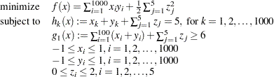The problem consists of a quadratic objective function, 1,000 linear equality constraints, and a linear inequality constraint. There are also 2,005 variables. You want to find a local minimum. To achieve this, you write the following statements:

proc optmodel;
   number n = 1000;
   number b = 5;
   var x{1..n} >=  - 1 <= 1 init 0.99;
   var y{1..n} >=  - 1 <= 1 init  - 0.99;
   var z{1..b} >= 0 <= 2 init 0.5;
   minimize f = sum {i in 1..n} x[i] * y[i]  + sum {j in 1..b} 0.5 * z[j]^2 ;
   con cons1: sum {i in 1..n} (x[i]  + y[i])  + sum {j in 1..b} z[j] >= b + 1;
   con cons2{i in 1..n}: x[i]  + y[i]  + sum {j in 1..b} z[j] = b;

   solve with IPNLP / tech=IPKRYLOV printfreq=10;
quit;

Note that this problem contains several thousands of variables and constraints. It is recommended that you use the TECH=IPKRYLOV option to obtain fast convergence for large-scale problems. The SAS output displays a detailed summary of the problem, together with the status of the solver at termination, the total number of iterations required, and the value of the objective function at the local minimum. The summaries and the optimal solution are shown in Output 9.3.

Figure 9.3 Problem Summary and the Optimal Solution

The OPTMODEL Procedure

Problem Summary
Objective Sense	Minimization
Objective Function	f
Objective Type	Quadratic

Number of Variables	2005
Bounded Above	0
Bounded Below	0
Bounded Below and Above	2005
Free	0
Fixed	0

Number of Constraints	1001
Linear LE (<=)	0
Linear EQ (=)	1000
Linear GE (>=)	1
Linear Range	0

Solution Summary
Solver	IPNLP/IPKRYLOV
Objective Function	f
Solution Status	Optimal
Objective Value	-996.4973658
Iterations	69

Optimality Error	6.2531155E-7
Infeasibility	2.3827055E-7

The SAS log shown in Output 9.4 displays a brief summary of the problem that is being solved, followed by the iterations generated by the solver.

Figure 9.4 Progress of the Algorithm As Shown in the Log

line

NOTE: The problem has 2005 variables (0 free, 0 fixed).
NOTE: The problem has 1001 linear constraints (0 LE, 1000 EQ, 1 GE, 0 range).
NOTE: The problem has 9005 linear constraint coefficients.
NOTE: The problem has 0 nonlinear constraints (0 LE, 0 EQ, 0 GE, 0 range).
NOTE: The OPTMODEL presolver removed 0 variables, 0 linear constraints, and 0
nonlinear constraints.
NOTE: Using analytic derivatives for objective.
NOTE: Using 2 threads for nonlinear evaluation.
NOTE: The Iterative Interior Point (IPKRYLOV) algorithm is called.
Objective Optimality
Iter Value Infeasibility Error
0 -979.47500000 2.25000000 2.25000000
10 -996.47961448 0.00033039 0.86685796
16 -996.50029947 0.0000000996945 0.0000000996945
NOTE: Converged.
NOTE: Objective = -996.500299.

Top of Page