| The NLPC Nonlinear Optimization Solver |
| Conditions of Optimality |
To facilitate discussion of the optimality conditions, we rewrite the general form of nonlinear optimization problems from the section Overview: NLPC Nonlinear Optimization Solver by grouping the equality constraints and inequality constraints. We also rewrite all the general nonlinear inequality constraints and bound constraints in one form as " " inequality constraints. Thus we have the following formulation:
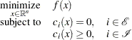 |
where  is the set of indices of the equality constraints,
  is the set of indices of the inequality constraints, and
  .
.
A point  is feasible if it satisfies all the constraints
  and
and  . The feasible region
  consists of all the feasible points. In unconstrained cases, the feasible region is the entire
  space.
A feasible point  is a local solution of the problem if there exists a neighborhood
  of such that
 |
Further, a feasible point is a strict local solution if strict inequality holds in the preceding case; i.e.,
 |
A feasible point is a global solution of the problem if no point in has a smaller function value than  ); i.e.,
 |
All the algorithms in the NLPC solver find a local solution of an optimization problem.
Unconstrained Optimization
The following conditions hold true for unconstrained optimization problems:
First-order necessary conditions: If
is a local solution and  is continuously differentiable in some neighborhood of , then
Second-order necessary conditions: If
is a local solution and is twice continuously differentiable in some neighborhood of , then  is positive semidefinite.
 Second-order sufficient conditions: If
is twice continuously differentiable in some neighborhood of ,  , and is positive definite, then is a strict local solution.
Constrained Optimization
For constrained optimization problems, the Lagrangian function is defined as follows:
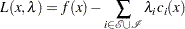 |
where  , are called Lagrange multipliers.
  is used to denote the gradient of the Lagrangian function with respect to , and
  is used to denote the Hessian of the Lagrangian function with respect to . The active set at a feasible point is defined as
 |
We also need the following definition before we can state the first-order and second-order necessary conditions:
Linear independence constraint qualification and regular point: A point
is said to satisfy the linear independence constraint qualification if the gradients of active constraints 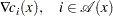
are linearly independent. Further, we refer to such a point
as a regular point.
We now state the theorems that are essential in the analysis and design of algorithms for constrained optimization:
First-order necessary conditions: Suppose that
is a local minimum and also a regular point. If and  , are continuously differentiable, there exist Lagrange multipliers
  such that the following conditions hold:

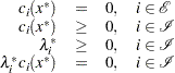
The preceding conditions are often known as the Karush-Kuhn-Tucker conditions, or KKT conditions for short. Also, the first set of equations are referred to as the stationarity condition, and the last set of equations are referred to as the complementarity condition.
Second-order necessary conditions: Suppose
is a local minimum and also a regular point. Let  be the Lagrange multipliers that satisfy the KKT conditions. If and
  , are twice continuously differentiable, the following conditions hold:
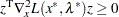
for all
 that satisfy
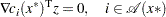
Second-order sufficient conditions: Suppose there exist a point
and some Lagrange multipliers such that the KKT conditions are satisfied. If the conditions 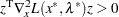
for all
that satisfy 
hold true, then
is a strict local solution. Note that the set of all such
 ’s forms the null space of the matrix
 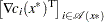 . Hence we can search for strict local solutions by numerically checking the Hessian of the Lagrangian function projected onto the null space. For a rigorous treatment of the optimality conditions, see Fletcher (1987) and Nocedal and Wright (1999).
The optimization algorithms in the NLPC solver apply an iterative process that results in a sequence of points,  , that converge to a local solution satisfying the first-order conditions. At the solution the NLPC solver performs tests to confirm that the second-order conditions are also satisfied.
Copyright © SAS Institute, Inc. All Rights Reserved.