Previous Page

|

Next Page

Example 13.4: Using the PENALTY= Option

The PENALTY= option plays an important role in ensuring a good convergence rate. Consider the following example:

Assume the starting point . You can use the following SAS code to solve the problem:

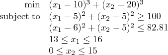
    proc optmodel;
       var x1 >=13 <=16, x2 >=0 <=15;
       
       minimize obj = 
          (x1-10)^3 + (x2-20)^3;
       
       con cons1:
          (x1-5)^2 + (x2-5)^2 - 100 >= 0;
       con cons2:
          82.81 - (x1-6)^2 - (x2-5)^2 >= 0;
       
       /* starting point */
       x1 = 14.35;
       x2 = 8.6;
       
       solve with sqp / printfreq = 5;
       print x1 x2;
    quit;
 

The optimal solution is displayed in Output 13.4.1.

The SQP solver might converge to the optimal solution more quickly if you specify PENALTY = 0.1 instead of the default value (0.75). You can specify the PENALTY= option in the SOLVE statement as follows:

  
    proc optmodel; 
    ... 
       solve with sqp / printfreq=5 penalty=0.1; 
    ... 
    quit;
 

The optimal solution is displayed in Output 13.4.2.

The iteration log is shown in Output 13.4.3.

You can see from Output 13.4.2 that the SQP solver took fewer iterations to converge to the optimal solution (see Output 13.4.1).