The Quadratic Programming Solver -- Experimental

Getting Started

Consider a small illustrative example. Suppose you want to minimize a two-variable quadratic function on the nonnegative quadrant, subject to two constraints:

$\min & 2x_1 & + & 3x_2 & + & x_1^2 & + & 10x_2^2 & + & 2.5 x_1 x_2 \ {subject ... ...& 100 & & & & \ & x_1 & & & \ge & 0 & & & & \ & & & x_2 & \ge & 0 & & & &$

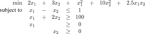
To use the OPTMODEL procedure, it is not necessary to fit this problem into the general QP formulation mentioned in the section "Overview" and to compute the corresponding parameters. However, since these parameters are closely related to the QPS-format data set, which is used by the OPTQP procedure, we compute these parameters for illustrative purposes as follows. The linear objective function coefficients, vector of right-hand sides, and lower and upper bounds are identified immediately as

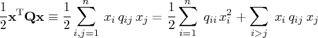
$\mathbf{c} = [2 \ 3 ], \mathbf{b} = [1 \ 100 ], \mathbf{l} = [0 \ 0 ], \mathbf{u} = [+\infty \ +\infty ]$

Let us carefully construct the quadratic matrix $\mathbf{q}$ . Observe that you can use symmetry to separate the main-diagonal and off-diagonal elements:

$\frac{1}2 \mathbf{x}^{\rm t} \mathbf{qx} \equiv \frac{1}2 \sum_{i, j = 1}^n\; ... ...\frac{1}2 \sum_{i = 1}^n\; q_{ii}\, x_i^2 + \sum_{i \gt j}\; x_i\, q_{ij}\, x_j$

The first expression

$\frac{1}2 \sum_{i = 1}^n\; q_{ii}\, x_i^2$

sums the main-diagonal elements. Thus in this case you have

$q_{11} = 2, q_{22} = 20$

Notice that the main-diagonal values are doubled in order to accommodate the 1/2 factor. Now the second term

$\sum_{i \gt j} x_i\, q_{ij}\, x_j$

sums the off-diagonal elements in the strict lower triangular part of the matrix. The only off-diagonal ( $x_i\, x_j,\; i\not=j$ ) term in the objective function is $2.5\, x_1\, x_2$ , so you have

$q_{21} = 2.5$

Notice that you do not need to specify the upper triangular part of the quadratic matrix.

Finally, the matrix of constraints is as follows:

$\mathbf{a} = [1 & -1 \ 1 & 2 ]$

The following OPTMODEL program formulates the preceding problem in a manner that is very close to the mathematical specification of the given problem.

    /* getting started */
    proc optmodel;
       var x1 >= 0; /* declare nonnegative variable x1 */
       var x2 >= 0; /* declare nonnegative variable x2 */
       
       /* objective: quadratic function f(x1, x2) */
       minimize f =
           /* the linear objective function coefficients */
           2 * x1 + 3 * x2 +
       
           /* quadratic <x, Qx> */
           x1 * x1 + 2.5 * x1 * x2 + 10 * x2 * x2;
       
       /* subject to the following constraints */
       con r1: x1 - x2 <= 1;
       con r2: x1 + 2 * x2 >= 100;
       
       /* specify iterative interior point algorithm (QP)
        * in the SOLVE statement */
       solve with qp;
       
       /* print the optimal solution */
       print x1 x2;
       save qps qpsdata;
    quit;

The "with qp" clause in the SOLVE statement invokes the QP solver to solve the problem. The output is shown in Output 12.2.

The OPTMODEL Procedure

Problem Summary
Objective Sense	Minimization
Objective Function	f
Objective Type	Quadratic

Number of Variables	2
Bounded Above	0
Bounded Below	2
Bounded Below and Above	0
Free	0
Fixed	0

Number of Constraints	2
Linear LE (<=)	1
Linear EQ (=)	0
Linear GE (>=)	1
Linear Range	0

The OPTMODEL Procedure

Solution Summary
Solver	QP
Objective Function	f
Solution Status	Optimal
Objective Value	15018.000761
Iterations	10

Primal Infeasibility	0
Dual Infeasibility	0
Bound Infeasibility	0
Duality Gap	9.9575984E-8
Complementarity	0.0014952645

x1	x2
34	33

Figure 12.2: Summaries and Optimal Solution

In this example, the SAVE QPS statement is used to save the QP problem in the QPS-format data set qpsdata, shown in Output 12.3. The data set is consistent with the parameters of general quadratic programming previously computed. Also, the data set can be used as input to the OPTQP procedure.

Obs	FIELD1	FIELD2	FIELD3	FIELD4	FIELD5	FIELD6
1	NAME		qpsdata	.		.
2	ROWS			.		.
3	N	f		.		.
4	L	r1		.		.
5	G	r2		.		.
6	COLUMNS			.		.
7		x1	f	2.0	r1	1
8		x1	r2	1.0		.
9		x2	f	3.0	r1	-1
10		x2	r2	2.0		.
11	RHS			.		.
12		.RHS.	r1	1.0		.
13		.RHS.	r2	100.0		.
14	QSECTION			.		.
15		x1	x1	2.0		.
16		x1	x2	2.5		.
17		x2	x2	20.0		.
18	ENDATA			.		.

Figure 12.3: QPS-Format Data Set

Top of Page