PROC OPTMODEL: Conditions of Optimality :: SAS/OR(R) 9.2 User's Guide: Mathematical Programming

The OPTMODEL Procedure

Conditions of Optimality

Linear Programming

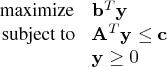
A standard linear program has the following formulation:

$\displaystyle\mathop\textrm{minimize}& \mathbf{c}^t \mathbf{x} \ \textrm{subject to}& \mathbf{a} \mathbf{x} \ge \mathbf{b} \ & \mathbf{x} \ge 0$

where

$\mathbf{x}$	$\in$	$\mathbb{r}^n$	is the vector of decision variables
$\mathbf{a}$	$\in$	$\mathbb{r}^{m x n}$	is the matrix of constraints
$\mathbf{c}$	$\in$	$\mathbb{r}^n$	is the vector of objective function coefficients
$\mathbf{b}$	$\in$	$\mathbb{r}^m$	is the vector of constraints right-hand sides (RHS)

This formulation is called the primal problem. The corresponding dual problem (see the section "Dual Values") is

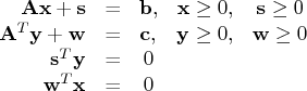
$\displaystyle\mathop\textrm{maximize}& \mathbf{b}^t \mathbf{y} \ \textrm{subject to}& \mathbf{a}^t \mathbf{y} \le \mathbf{c} \ & \mathbf{y} \ge 0$

where $\mathbf{y} \in \mathbb{r}^m$ is the vector of dual variables.

The vectors $\mathbf{x}$ and $\mathbf{y}$ are optimal to the primal and dual problems, respectively, only if there exist primal slack variables $\mathbf{s} = \mathbf{a} \mathbf{x} - \mathbf{b}$ and dual slack variables $\mathbf{w} = \mathbf{a}^t \mathbf{y} - \mathbf{c}$ such that the following Karush-Kuhn-Tucker (KKT) conditions are satisfied:

$\mathbf{a} \mathbf{x} + \mathbf{s} & = & \mathbf{b}, & \mathbf{x} \ge 0, & \math... ...e 0 \ \mathbf{s}^t \mathbf{y} & = & 0 \ \mathbf{w}^t \mathbf{x} & = & 0 \$

The first line of equations defines primal feasibility, the second line of equations defines dual feasibility, and the last two equations are called the complementary slackness conditions.

Nonlinear Programming

To facilitate discussion of optimality conditions in nonlinear programming, we write the general form of nonlinear optimization problems by grouping the equality constraints and inequality constraints. We also write all the general nonlinear inequality constraints and bound constraints in one form as `` $\ge$ '' inequality constraints. Thus we have the following formulation:

$\displaystyle\mathop\textrm{minimize}_{x\in{\mathbb r}^n} & f(x) \ \textrm{subject to}& c_i(x) = 0, & i \in {\cal e} \ & c_i(x) \ge 0, & i \in {\cal i}$

where $\cal e$ is the set of indices of the equality constraints, $\cal i$ is the set of indices of the inequality constraints, and $m=|{\cal e}|+|{\cal i}|$ .

A point is feasible if it satisfies all the constraints $c_i(x) = 0, i\in{\cal e}$ and $c_i(x) \ge 0, i\in{\cal i}$ . The feasible region ${\cal f}$ consists of all the feasible points. In unconstrained cases, the feasible region ${\cal f}$ is the entire $\mathbb{r}^n$ space.

A feasible point is a local solution of the problem if there exists a neighborhood ${\cal n}$ of such that

$f(x)\ge f(x^*)\;\;{\rm forall} x\in{\cal n}\cap{\cal f}$

Further, a feasible point

is a strict local solution if strict inequality holds in the preceding case; i.e.,

$f(x) \gt f(x^*)\;\;{\rm forall} x\in{\cal n}\cap{\cal f}$

A feasible point

is a global solution of the problem if no point in ${\cal f}$ has a smaller function value than

); i.e.,

$f(x)\ge f(x^*)\;\; {\rm for all } x\in{\cal f}$

Unconstrained Optimization

The following conditions hold true for unconstrained optimization problems:

First-order necessary conditions: If is a local solution and is continuously differentiable in some neighborhood of , then
$\nabla\!f(x^*) = 0$
Second-order necessary conditions: If is a local solution and is twice continuously differentiable in some neighborhood of , then $\nabla^2\!f(x^*)$ is positive semidefinite.
Second-order sufficient conditions: If is twice continuously differentiable in some neighborhood of , $\nabla\!f(x^*) = 0$ , and $\nabla^2\!f(x^*)$ is positive definite, then is a strict local solution.

Constrained Optimization

For constrained optimization problems, the Lagrangian function is defined as follows:

$l(x,\lambda) = f(x) - \sum_{i\in{\cal e}\cup{\cal i}} \lambda_i c_i(x)$

where $\lambda_i,i\in{\cal e}\cup{\cal i}$ , are called Lagrange multipliers. $\nabla\!_x l(x,\lambda)$ is used to denote the gradient of the Lagrangian function with respect to

, and $\nabla_{\!x}^2 l(x,\lambda)$ is used to denote the Hessian of the Lagrangian function with respect to

. The active set at a feasible point

is defined as

${\cal a}(x)={\cal e}\cup\{i\in{\cal i}: c_i(x)=0\}$

We also need the following definition before we can state the first-order and second-order necessary conditions:

Linear independence constraint qualification and regular point: A point is said to satisfy the linear independence constraint qualification if the gradients of active constraints
$\nabla\!c_i(x), i\in{\cal a}(x)$
are linearly independent. Further, we refer to such a point as a regular point .

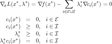
We now state the theorems that are essential in the analysis and design of algorithms for constrained optimization:

First-order necessary conditions: Suppose that is a local minimum and also a regular point. If and $c_i(x),i \in{\cal e}\cup{\cal i}$ , are continuously differentiable, there exist Lagrange multipliers $\lambda^*\in{\mathbb r}^m$ such that the following conditions hold:
$& & \;\:\nabla\!_x l(x^*,\lambda^*) = \nabla\!f(x^*)-\displaystyle\mathop{\sum}_... ...^* & \ge & 0, & i\in{\cal i} \ \lambda_i^* c_i(x^*) & = & 0, & i\in{\cal i}$
The preceding conditions are often known as the Karush-Kuhn-Tucker conditions, or KKT conditions for short.
Second-order necessary conditions: Suppose that is a local minimum and also a regular point. Let $\lambda^*$ be the Lagrange multipliers that satisfy the KKT conditions. If and $c_i(x),i \in{\cal e}\cup{\cal i}$ , are twice continuously differentiable, the following conditions hold:
$z^t \nabla_{\!x}^2 l(x^*,\lambda^*)z \ge 0$
for all $z\in{\mathbb r}^n$ that satisfy
$\nabla\!c_i(x^*)^tz = 0, i\in{\cal a}(x^{*})$
Second-order sufficient conditions: Suppose there exist a point and some Lagrange multipliers $\lambda^*$ such that the KKT conditions are satisfied. If
$z^t \nabla_{\!x}^2 l(x^*,\lambda^*)z \gt 0$
for all $z\in{\mathbb r}^n$ that satisfy
$\nabla\!c_i(x^*)^tz = 0, i\in{\cal a}(x^{*})$
then is a strict local solution.

Note that the set of all such 's forms the null space of the matrix $[\nabla\!c_i(x^*)^t ]_{i\in{\cal a}(x^{*})}$ . Thus we can search for strict local solutions by numerically checking the Hessian of the Lagrangian function projected onto the null space. For a rigorous treatment of the optimality conditions, see Fletcher (1987) and Nocedal and Wright (1999).

Top of Page