PROC NLP: Active Set Methods :: SAS/OR(R) 9.2 User's Guide: Mathematical Programming

The NLP Procedure

Active Set Methods

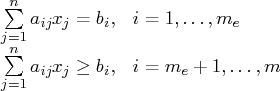
The parameter vector $x \in {\cal r}^n$ may be subject to a set of linear equality and inequality constraints:

$\sum\limits_{j=1}^n a_{ij} x_j = b_i, & i=1, ... , m_e \ \sum\limits_{j=1}^n a_{ij} x_j \geq b_i, & i=m_e+1, ... , m$

The coefficients $a_{ij}$ and right-hand sides

of the equality and inequality constraints are collected in the

matrix

and the

vector

The linear constraints define a feasible region ${\cal g}$ in ${\cal r}^n$ that must contain the point $x^{*}$ that minimizes the problem. If the feasible region ${\cal g}$ is empty, no solution to the optimization problem exists.

All optimization techniques in PROC NLP (except those processing nonlinear constraints) are active set methods. The iteration starts with a feasible point $x^{(0)}$ , which either is provided by the user or can be computed by the Schittkowski and Stoer (1979) algorithm implemented in PROC NLP. The algorithm then moves from one feasible point $x^{(k-1)}$ to a better feasible point $x^{(k)}$ along a feasible search direction $s^{(k)}$ :

$x^{(k)} = x^{(k-1)} + \alpha^{(k)} s^{(k)} \:, \alpha^{(k)} \gt 0$

Theoretically, the path of points $x^{(k)}$ never leaves the feasible region ${\cal g}$ of the optimization problem, but it can hit its boundaries. The active set ${\cal a}^{(k)}$ of point $x^{(k)}$ is defined as the index set of all linear equality constraints and those inequality constraints that are satisfied at $x^{(k)}$ . If no constraint is active for $x^{(k)}$ , the point is located in the interior of ${\cal g}$ , and the active set ${\cal a}^{(k)}$ is empty. If the point $x^{(k)}$ in iteration hits the boundary of inequality constraint , this constraint becomes active and is added to ${\cal a}^{(k)}$ . Each equality or active inequality constraint reduces the dimension (degrees of freedom) of the optimization problem.

In practice, the active constraints can be satisfied only with finite precision. The LCEPSILON= option specifies the range for active and violated linear constraints. If the point $x^{(k)}$ satisfies the condition

$| \sum_{j=1}^n a_{ij} x_j^{(k)} - b_i | \leq t$

where

, the constraint

is recognized as an active constraint. Otherwise, the constraint

is either an inactive inequality or a violated inequality or equality constraint. Due to rounding errors in computing the projected search direction, error can be accumulated so that an iterate $x^{(k)}$ steps out of the feasible region. In those cases, PROC NLP may try to pull the iterate $x^{(k)}$ into the feasible region. However, in some cases the algorithm needs to increase the feasible region by increasing the LCEPSILON=

value. If this happens it is indicated by a message displayed in the log output.

If you cannot expect an improvement in the value of the objective function by moving from an active constraint back into the interior of the feasible region, you use this inequality constraint as an equality constraint in the next iteration. That means the active set ${\cal a}^{(k+1)}$ still contains the constraint . Otherwise you release the active inequality constraint and increase the dimension of the optimization problem in the next iteration.

A serious numerical problem can arise when some of the active constraints become (nearly) linearly dependent. Linearly dependent equality constraints are removed before entering the optimization. You can use the LCSINGULAR= option to specify a criterion used in the update of the QR decomposition that decides whether an active constraint is linearly dependent relative to a set of other active constraints.

If the final parameter set $x^{*}$ is subjected to $n_{act}$ linear equality or active inequality constraints, the QR decomposition of the $n x n_{act}$ matrix $\hat{a}^t$ of the linear constraints is computed by $\hat{a}^t = qr$ , where is an orthogonal matrix and is an $n x n_{act}$ upper triangular matrix. The columns of matrix can be separated into two matrices, , where contains the first $n_{act}$ orthogonal columns of and contains the last $n-n_{act}$ orthogonal columns of . The $n x (n-n_{act})$ column-orthogonal matrix is also called the nullspace matrix of the active linear constraints $\hat{a}^t$ . The $n-n_{act}$ columns of the $n x (n-n_{act})$ matrix form a basis orthogonal to the rows of the $n_{act} x n$ matrix $\hat{a}$ .

At the end of the iteration process, the PROC NLP can display the projected gradient

In the case of boundary constrained optimization, the elements of the projected gradient correspond to the gradient elements of the free parameters. A necessary condition for $x^{*}$ to be a local minimum of the optimization problem is

$g_z(x^{*}) = z^tg(x^{*}) = 0$

The symmetric $n_{act} x n_{act}$ matrix

is called a projected Hessian matrix. A second-order necessary condition for $x^{*}$ to be a local minimizer requires that the projected Hessian matrix is positive semidefinite. If available, the projected gradient and projected Hessian matrix can be displayed and written in an OUTEST= data set.

Those elements of the $n_{act}$ vector of first-order estimates of Lagrange multipliers

$\lambda = (\hat{a}\hat{a}^t)^{-1} \hat{a} zz^t g$

which correspond to active inequality constraints indicate whether an improvement of the objective function can be obtained by releasing this active constraint. For minimization (maximization), a significant negative (positive) Lagrange multiplier indicates that a possible reduction (increase) of the objective function can be obtained by releasing this active linear constraint. The LCDEACT=

option can be used to specify a threshold

for the Lagrange multiplier that decides whether an active inequality constraint remains active or can be deactivated. The Lagrange multipliers are displayed (and written in an OUTEST= data set) only if linear constraints are active at the solution $x^{*}$ . (In the case of boundary-constrained optimization, the Lagrange multipliers for active lower (upper) constraints are the negative (positive) gradient elements corresponding to the active parameters.)

Top of Page