PROC NETFLOW: RESET Statement :: SAS/OR(R) 9.2 User's Guide: Mathematical Programming

The NETFLOW Procedure

RESET Statement

RESET options ;

SET options ;

The RESET statement is used to change options after PROC NETFLOW has started execution. Any of the following options can appear in the PROC NETFLOW statement.

Another name for the RESET statement is SET. You can use RESET when you are resetting options and SET when you are setting options for the first time.

The following options fall roughly into five categories:

output data set specifications
options that indicate conditions under which optimization is to be halted temporarily, giving you an opportunity to use PROC NETFLOW interactively
options that control aspects of the operation of the network primal simplex optimization
options that control the pricing strategies of the network simplex optimizer
miscellaneous options

If you want to examine the setting of any options, use the SHOW statement. If you are interested in looking at only those options that fall into a particular category, the SHOW statement has options that enable you to do this.

The execution of PROC NETFLOW has three stages. In stage zero the problem data are read from the NODEDATA=, ARCDATA=, and CONDATA= data sets. If a warm start is not available, an initial basic feasible solution is found. Some options of the PROC NETFLOW statement control what occurs in stage zero. By the time the first RESET statement is processed, stage zero has already been completed.

In the first stage, an optimal solution to the network flow problem neglecting any side constraints is found. The primal and dual solutions for this relaxed problem can be saved in the ARCOUT= data set and the NODEOUT= data set, respectively.

In the second stage, the side constraints are examined and some initializations occur. Some preliminary work is also needed to commence optimization that considers the constraints. An optimal solution to the network flow problem with side constraints is found. The primal and dual solutions for this side-constrained problem are saved in the CONOUT= data set and the DUALOUT= data set, respectively.

Many options in the RESET statement have the same name except that they have as a suffix the numeral 1 or 2. Such options have much the same purpose, but option1 controls what occurs during the first stage when optimizing the network neglecting any side constraints and option2 controls what occurs in the second stage when PROC NETFLOW is performing constrained optimization.

Some options can be turned off by the option prefixed by the word NO. For example, FEASIBLEPAUSE1 may have been specified in a RESET statement and in a later RESET statement, you can specify NOFEASIBLEPAUSE1. In a later RESET statement, you can respecify FEASIBLEPAUSE1 and, in this way, toggle this option.

The options available with the RESET statement are summarized by purpose in the following table.

Table 5.3: Functional Summary, RESET Statement

Description	Statement	Option
Output Data Set Options:
unconstrained primal solution data set	RESET	ARCOUT=
unconstrained dual solution data set	RESET	NODEOUT=
constrained primal solution data set	RESET	CONOUT=
constrained dual solution data set	RESET	DUALOUT=

Simplex Options:
use big-M instead of two-phase method, stage 1	RESET	BIGM1
use Big-M instead of two-phase method, stage 2	RESET	BIGM2
anti-cycling option	RESET	CYCLEMULT1=
interchange first nonkey with leaving key arc	RESET	INTFIRST
controls working basis matrix inversions	RESET	INVFREQ=
maximum number of L row operations allowed before refactorization	RESET	MAXL=
maximum number of LU factor column updates	RESET	MAXLUUPDATES=
anti-cycling option	RESET	MINBLOCK1=
use first eligible leaving variable, stage 1	RESET	LRATIO1
use first eligible leaving variable, stage 2	RESET	LRATIO2
negates INTFIRST	RESET	NOINTFIRST
negates LRATIO1	RESET	NOLRATIO1
negates LRATIO2	RESET	NOLRATIO2
negates PERTURB1	RESET	NOPERTURB1
anti-cycling option	RESET	PERTURB1
controls working basis matrix refactorization	RESET	REFACTFREQ=
use two-phase instead of big-M method, stage 1	RESET	TWOPHASE1
use two-phase instead of big-M method, stage 2	RESET	TWOPHASE2
pivot element selection parameter	RESET	U=
zero tolerance, stage 1	RESET	ZERO1=
zero tolerance, stage 2	RESET	ZERO2=
zero tolerance, real number comparisons	RESET	ZEROTOL=

Pricing Options:
frequency of dual value calculation	RESET	DUALFREQ=
pricing strategy, stage 1	RESET	PRICETYPE1=
pricing strategy, stage 2	RESET	PRICETYPE2=
used when P1SCAN=PARTIAL	RESET	P1NPARTIAL=
controls search for entering candidate, stage 1	RESET	P1SCAN=
used when P2SCAN=PARTIAL	RESET	P2NPARTIAL=
controls search for entering candidate, stage 2	RESET	P2SCAN=
initial queue size, stage 1	RESET	QSIZE1=
initial queue size, stage 2	RESET	QSIZE2=
used when Q1FILLSCAN=PARTIAL	RESET	Q1FILLNPARTIAL=
controls scan when filling queue, stage 1	RESET	Q1FILLSCAN=
used when Q2FILLSCAN=PARTIAL	RESET	Q2FILLNPARTIAL=
controls scan when filling queue, stage 2	RESET	Q2FILLSCAN=
queue size reduction factor, stage 1	RESET	REDUCEQSIZE1=
queue size reduction factor, stage 2	RESET	REDUCEQSIZE2=
frequency of refreshing queue, stage 1	RESET	REFRESHQ1=
frequency of refreshing queue, stage 2	RESET	REFRESHQ2=

Optimization Termination Options:
pause after stage 1; don't start stage 2	RESET	ENDPAUSE1
pause when feasible, stage 1	RESET	FEASIBLEPAUSE1
pause when feasible, stage 2	RESET	FEASIBLEPAUSE2
maximum number of iterations, stage 1	RESET	MAXIT1=
maximum number of iterations, stage 2	RESET	MAXIT2=
negates ENDPAUSE1	RESET	NOENDPAUSE1
negates FEASIBLEPAUSE1	RESET	NOFEASIBLEPAUSE1
negates FEASIBLEPAUSE2	RESET	NOFEASIBLEPAUSE2
pause every PAUSE1 iterations, stage 1	RESET	PAUSE1=
pause every PAUSE2 iterations, stage 2	RESET	PAUSE2=

Interior Point Algorithm Options:
factorization method	RESET	FACT_METHOD=
allowed amount of dual infeasibility	RESET	TOLDINF=
allowed amount of primal infeasibility	RESET	TOLPINF=
allowed total amount of dual infeasibility	RESET	TOLTOTDINF=
allowed total amount of primal infeasibility	RESET	TOLTOTPINF=
cut-off tolerance for Cholesky factorization	RESET	CHOLTINYTOL=
density threshold for Cholesky processing	RESET	DENSETHR=
step-length multiplier	RESET	PDSTEPMULT=
preprocessing type	RESET	PRSLTYPE=
print optimization progress on SAS log	RESET	PRINTLEVEL2=

Interior Point Stopping Criteria Options:
maximum number of interior point iterations	RESET	MAXITERB=
primal-dual (duality) gap tolerance	RESET	PDGAPTOL=
stop because of complementarity	RESET	STOP_C=
stop because of duality gap	RESET	STOP_DG=
stop because of ${infeas}_b$	RESET	STOP_IB=
stop because of ${infeas}_c$	RESET	STOP_IC=
stop because of ${infeas}_d$	RESET	STOP_ID=
stop because of complementarity	RESET	AND_STOP_C=
stop because of duality gap	RESET	AND_STOP_DG=
stop because of ${infeas}_b$	RESET	AND_STOP_IB=
stop because of ${infeas}_c$	RESET	AND_STOP_IC=
stop because of ${infeas}_d$	RESET	AND_STOP_ID=
stop because of complementarity	RESET	KEEPGOING_C=
stop because of duality gap	RESET	KEEPGOING_DG=
stop because of ${infeas}_b$	RESET	KEEPGOING_IB=
stop because of ${infeas}_c$	RESET	KEEPGOING_IC=
stop because of ${infeas}_d$	RESET	KEEPGOING_ID=
stop because of complementarity	RESET	AND_KEEPGOING_C=
stop because of duality gap	RESET	AND_KEEPGOING_DG=
stop because of ${infeas}_b$	RESET	AND_KEEPGOING_IB=
stop because of ${infeas}_c$	RESET	AND_KEEPGOING_IC=
stop because of ${infeas}_d$	RESET	AND_KEEPGOING_ID=

Miscellaneous Options:
output complete basis information to ARCOUT= and NODEOUT= data sets	RESET	FUTURE1
output complete basis information to CONOUT= and DUALOUT= data sets	RESET	FUTURE2
turn off infeasibility or optimality flags	RESET	MOREOPT
negates FUTURE1	RESET	NOFUTURE1
negates FUTURE2	RESET	NOFUTURE2
negates SCRATCH	RESET	NOSCRATCH
negates ZTOL1	RESET	NOZTOL1
negates ZTOL2	RESET	NOZTOL2
write optimization time to SAS log	RESET	OPTIM_TIMER
no stage 1 optimization; do stage 2 optimization	RESET	SCRATCH
suppress similar SAS log messages	RESET	VERBOSE=
use zero tolerance, stage 1	RESET	ZTOL1
use zero tolerance, stage 2	RESET	ZTOL2

Output Data Set Specifications

In a RESET statement, you can specify an ARCOUT= data set, a NODEOUT= data set, a CONOUT= data set, or a DUALOUT= data set. You are advised to specify these output data sets early because if you make a syntax error when using PROC NETFLOW interactively or, for some other reason, PROC NETFLOW encounters or does something unexpected, these data sets will contain information about the solution that was reached. If you had specified the FUTURE1 or FUTURE2 option in a RESET statement, PROC NETFLOW may be able to resume optimization in a subsequent run.

You can turn off these current output data set specifications by specifying ARCOUT=NULL, NODEOUT=NULL, CONOUT=NULL, or DUALOUT=NULL.

If PROC NETFLOW is outputting observations to an output data set and you want this to stop, press the keys used to stop SAS procedures. PROC NETFLOW waits, if necessary, and then executes the next statement.

ARCOUT=SAS-data-set
AOUT=SAS-data-set: names the output data set that receives all information concerning arc and nonarc variables, including flows and other information concerning the current solution and the supply and demand information. The current solution is the latest solution found by the optimizer when the optimization neglecting side constraints is halted or the unconstrained optimum is reached.

You can specify an ARCOUT= data set in any RESET statement before the unconstrained optimum is found (even at commencement). Once the unconstrained optimum has been reached, use the SAVE statement to produce observations in an ARCOUT= data set. Once optimization that considers constraints starts, you will be unable to obtain an ARCOUT= data set. Instead, use a CONOUT= data set to get the current solution. See the section "ARCOUT= and CONOUT= Data Sets" for more information.
CONOUT=SAS-data-set
COUT=SAS-data-set: names the output data set that contains the primal solution obtained after optimization considering side constraints reaches the optimal solution. You can specify a CONOUT= data set in any RESET statement before the constrained optimum is found (even at commencement or while optimizing neglecting constraints). Once the constrained optimum has been reached, or during stage 2 optimization, use the SAVE statement to produce observations in a CONOUT= data set. See the section "ARCOUT= and CONOUT= Data Sets" for more information.
DUALOUT=SAS-data-set
DOUT=SAS-data-set: names the output data set that contains the dual solution obtained after doing optimization that considers side constraints reaches the optimal solution. You can specify a DUALOUT= data set in any RESET statement before the constrained optimum is found (even at commencement or while optimizing neglecting constraints). Once the constrained optimum has been reached, or during stage 2 optimization, use the SAVE statement to produce observations in a DUALOUT= data set. See the section "NODEOUT= and DUALOUT= Data Sets" for more information.
NODEOUT=SAS-data-set
NOUT=SAS-data-set: names the output data set that receives all information about nodes (supply/demand and nodal dual variable values) and other information concerning the unconstrained optimal solution.

You can specify a NODEOUT= data set in any RESET statement before the unconstrained optimum is found (even at commencement). Once the unconstrained optimum has been reached, or during stage 1 optimization, use the SAVE statement to produce observations in a NODEOUT= data set. Once optimization that considers constraints starts, you will not be able to obtain a NODEOUT= data set. Instead use a DUALOUT= data set to get the current solution. See the section "NODEOUT= and DUALOUT= Data Sets" for more information.

Options to Halt Optimization

The following options indicate conditions when optimization is to be halted. You then have a chance to use PROC NETFLOW interactively. If the NETFLOW procedure is optimizing and you want optimization to halt immediately, press the CTRL-BREAK key combination used to stop SAS procedures. Doing this is equivalent to PROC NETFLOW finding that some prespecified condition of the current solution under which optimization should stop has occurred.

If optimization does halt, you may need to change the conditions for when optimization should stop again. For example, if the number of iterations exceeded MAXIT2, use the RESET statement to specify a larger value for the MAXIT2= option before the next RUN statement. Otherwise, PROC NETFLOW will immediately find that the number of iterations still exceeds MAXIT2 and halt without doing any additional optimization.

ENDPAUSE1: indicates that PROC NETFLOW will pause after the unconstrained optimal solution has been obtained and information about this solution has been output to the current ARCOUT= data set, NODEOUT= data set, or both. The procedure then executes the next statement, or waits if no subsequent statement has been specified.
FEASIBLEPAUSE1
FP1: indicates that unconstrained optimization should stop once a feasible solution is reached. PROC NETFLOW checks for feasibility every 10 iterations. A solution is feasible if there are no artificial arcs having nonzero flow assigned to be conveyed through them. The presence of artificial arcs with nonzero flows means that the current solution does not satisfy all the nodal flow conservation constraints implicit in network problems.
MAXIT1=m: specifies the maximum number of primal simplex iterations PROC NETFLOW is to perform in stage 1. The default value for the MAXIT1= option is 1000. If MAXIT1=m iterations are performed and you want to continue unconstrained optimization, reset MAXIT1= to a number larger than the number of iterations already performed and issue another RUN statement.
NOENDPAUSE1
NOEP1: negates the ENDPAUSE1 option.
NOFEASIBLEPAUSE1
NOFP1: negates the FEASIBLEPAUSE1 option.
PAUSE1=p: indicates that PROC NETFLOW will halt unconstrained optimization and pause when the remainder of the number of stage 1 iterations divided by the value of the PAUSE1= option is zero. If present, the next statement is executed; if not, the procedure waits for the next statement to be specified. The default value for PAUSE1= is 999999.
FEASIBLEPAUSE2
FP2
NOFEASIBLEPAUSE2
NOFP2
PAUSE2=p
MAXIT2=m: are the stage 2 constrained optimization counterparts of the options described previously and having as a suffix the numeral 1.

Options Controlling the Network Simplex Optimization

BIGM1
NOTWOPHASE1
TWOPHASE1
NOBIGM1: BIGM1 indicates that the "big-M" approach to optimization is used. Artificial variables are treated like real arcs, slacks, surpluses and nonarc variables. Artificials have very expensive costs. BIGM1 is the default.

TWOPHASE1 indicates that the two-phase approach is used instead of the big-M approach. At first, artificial variables are the only variables to have nonzero objective function coefficients. An artificial variable's objective function coefficient is temporarily set to 1 and PROC NETFLOW minimizes. When all artificial variables have zero value, PROC NETFLOW has found a feasible solution, and phase 2 commences. Arcs and nonarc variables have their real costs and objective function coefficients.

Before all artificial variables are driven to have zero value, you can toggle between the big-M and the two-phase approaches by specifying BIGM1 or TWOPHASE1 in a RESET statement. The option NOTWOPHASE1 is synonymous with BIGM1, and NOBIGM1 is synonymous with TWOPHASE1.
CYCLEMULT1=c
MINBLOCK1=m
NOPERTURB1
PERTURB1: In an effort to reduce the number of iterations performed when the problem is highly degenerate, PROC NETFLOW has in stage 1 optimization adopted an algorithm outlined in Ryan and Osborne (1988).

If the number of consecutive degenerate pivots (those with no progress toward the optimum) performed equals the value of the CYCLEMULT1= option times the number of nodes, the arcs that were "blocking" (can leave the basis) are added to a list. In subsequent iterations, of the arcs that now can leave the basis, the one chosen to leave is an arc on the list of arcs that could have left in the previous iteration. In other words, perference is given to arcs that "block" many iterations. After several iterations, the list is cleared.

If the number of blocking arcs is less than the value of the MINBLOCK1= option, a list is not kept. Otherwise, if PERTURB1 is specified, the arc flows are perturbed by a random quantity, so that arcs on the list that block subsequent iterations are chosen to leave the basis randomly. Although perturbation often pays off, it is computationally expensive. Periodically, PROC NETFLOW has to clear out the lists and un-perturb the solution. You can specify NOPERTURB1 to prevent perturbation.

Defaults are CYCLEMULT1=0.15, MINBLOCK1=2, and NOPERTURB1.
LRATIO1: specifies the type of ratio test to use in determining which arc leaves the basis in stage 1. In some iterations, more than one arc is eligible to leave the basis. Of those arcs that can leave the basis, the leaving arc is the first encountered by the algorithm if the LRATIO1 option is specified. Specifying the LRATIO1 option can decrease the chance of cycling but can increase solution times. The alternative to the LRATIO1 option is the NOLRATIO1 option, which is the default.
LRATIO2: specifies the type of ratio test to use in determining what leaves the basis in stage 2. In some iterations, more than one arc, constraint slack, surplus, or nonarc variable is eligible to leave the basis. If the LRATIO2 option is specified, the leaving arc, constraint slack, surplus, or nonarc variable is the one that is eligible to leave the basis first encountered by the algorithm. Specifying the LRATIO2 option can decrease the chance of cycling but can increase solution times. The alternative to the LRATIO2 option is the NOLRATIO2 option, which is the default.
NOLRATIO1: specifies the type of ratio test to use in determining which arc leaves the basis in stage 1. If the NOLRATIO1 option is specified, of those arcs that can leave the basis, the leaving arc has the minimum (maximum) cost if the leaving arc is to be nonbasic with flow capacity equal to its capacity (lower flow bound). If more than one possible leaving arc has the minimum (maximum) cost, the first such arc encountered is chosen. Specifying the NOLRATIO1 option can decrease solution times, but can increase the chance of cycling. The alternative to the NOLRATIO1 option is the LRATIO1 option. The NOLRATIO1 option is the default.
NOLRATIO2: specifies the type of ratio test to use in determining which arc leaves the basis in stage 2. If the NOLRATIO2 option is specified, the leaving arc, constraint slack, surplus, or nonarc variable is the one eligible to leave the basis with the minimum (maximum) cost or objective function coefficient if the leaving arc, constraint slack or nonarc variable is to be nonbasic with flow or value equal to its capacity or upper value bound (lower flow or value bound), respectively. If several possible leaving arcs, constraint slacks, surpluses, or nonarc variables have the minimum (maximum) cost or objective function coefficient, then the first encountered is chosen. Specifying the NOLRATIO2 option can decrease solution times, but can increase the chance of cycling. The alternative to the NOLRATIO2 option is the LRATIO2 option. The NOLRATIO2 option is the default.

Options Applicable to Constrained Optimization

The INVFREQ= option is relevant only if INVD_2D is specified in the PROC NETFLOW statement; that is, the inverse of the working basis matrix is being stored and processed as a two-dimensional array. The REFACTFREQ=, U=, MAXLUUPDATES=, and MAXL= options are relevant if the INVD_2D option is not specified in the PROC NETFLOW statement; that is, if the working basis matrix is LU factored.

BIGM2
NOTWOPHASE2
TWOPHASE2
NOBIGM2: are the stage 2 constrained optimization counterparts of the options BIGM1, NOTWOPHASE1, TWOPHASE1, and NOBIGM1.

The TWOPHASE2 option is often better than the BIGM2 option when the problem has many side constraints.
INVFREQ=n: recalculates the working basis matrix inverse whenever n iterations have been performed where n is the value of the INVFREQ= option. Although a relatively expensive task, it is prudent to do as roundoff errors accumulate, especially affecting the elements of this matrix inverse. The default is INVFREQ=50. The INVFREQ= option should be used only if the INVD_2D option is specified in the PROC NETFLOW statement.
INTFIRST: In some iterations, it is found that what must leave the basis is an arc that is part of the spanning tree representation of the network part of the basis (called a key arc). It is necessary to interchange another basic arc not part of the tree (called a nonkey arc) with the tree arc that leaves to permit the basis update to be performed efficiently. Specifying the INTFIRST option indicates that of the nonkey arcs eligible to be swapped with the leaving key arc, the one chosen to do so is the first encountered by the algorithm. If the INTFIRST option is not specified, all such arcs are examined and the one with the best cost is chosen.

The terms key and nonkey are used because the algorithm used by PROC NETFLOW for network optimization considering side constraints (GUB-based, Primal Partitioning, or Factorization) is a variant of an algorithm originally developed to solve linear programming problems with generalized upper bounding constraints. The terms key and nonkey were coined then. The STATUS SAS variable in the ARCOUT= and CONOUT= data sets and the STATUS column in tables produced when PRINT statements are processed indicate whether basic arcs are key or nonkey. Basic nonarc variables are always nonkey.
MAXL=m: If the working basis matrix is LU factored, U is an upper triangular matrix and L is a lower triangular matrix corresponding to a sequence of elementary matrix row operations required to change the working basis matrix into U. L and U enable substitution techniques to be used to solve the linear systems of the simplex algorithm. Among other things, the LU processing strives to keep the number of L elementary matrix row operation matrices small. A buildup in the number of these could indicate that fill-in is becoming excessive and the computations involving L and U will be hampered. Refactorization should be performed to restore U sparsity and reduce L information. When the number of L matrix row operations exceeds the value of the MAXL= option, a refactorization is done rather than one or more updates. The default value for MAXL= is 10 times the number of side constraints. The MAXL= option should not be used if INVD_2D is specified in the PROC NETFLOW statement.
MAXLUUPDATES=m
MLUU=m: In some iterations, PROC NETFLOW must either perform a series of single column updates or a complete refactorization of the working basis matrix. More than one column of the working basis matrix must change before the next simplex iteration can begin. The single column updates can often be done faster than a complete refactorization, especially if few updates are necessary, the working basis matrix is sparse, or a refactorization has been performed recently. If the number of columns that must change is less than the value specified in the MAXLUUPDATES= option, the updates are attempted; otherwise, a refactorization is done. Refactorization also occurs if the sum of the number of columns that must be changed and the number of LU updates done since the last refactorization exceeds the value of the REFACTFREQ= option. The MAXLUUPDATES= option should not be used if the INVD_2D option is specified in the PROC NETFLOW statement.

In some iterations, a series of single column updates are not able to complete the changes required for a working basis matrix because, ideally, all columns should change at once. If the update cannot be completed, PROC NETFLOW performs a refactorization. The default value is 5.
NOINTFIRST: indicates that of the arcs eligible to be swapped with the leaving arc, the one chosen to do so has the best cost. See the INTFIRST option.
REFACTFREQ=r
RFF=r: specifies the maximum number of L and U updates between refactorization of the working basis matrix to reinitialize LU factors. In most iterations, one or several Bartels-Golub updates can be performed. An update is performed more quickly than a complete refactorization. However, after a series of updates, the sparsity of the U factor is degraded. A refactorization is necessary to regain sparsity and to make subsequent computations and updates more efficient. The default value is 50. The REFACTFREQ= option should not be used if INVD_2D is specified in the PROC NETFLOW statement.
U=u: controls the choice of pivot during LU decomposition or Bartels-Golub update. When searching for a pivot, any element less than the value of the U= option times the largest element in its matrix row is excluded, or matrix rows are interchanged to improve numerical stability. The U= option should have values on or between ZERO2 and 1.0. Decreasing the value of the U= option biases the algorithm toward maintaining sparsity at the expense of numerical stability and vice-versa. Reid (1975) suggests that the value of 0.01 is acceptable and this is the default for the U= option. This option should not be used if INVD_2D is specified in the PROC NETFLOW statement.

Pricing Strategy Options

There are three main types of pricing strategies:

PRICETYPE=NOQ
PRICETYPE=BLAND
PRICETYPE=Q

The one that usually performs better than the others is PRICETYPE

=Q, so this is the default.

Because the pricing strategy takes a lot of computational time, you should experiment with the following options to find the optimum specification. These options influence how the pricing step of the simplex iteration is performed. See the section "Pricing Strategies" for further information.

PRICETYPE

=BLAND or PTYPE

=BLAND

PRICETYPE

=NOQ or PTYPE

=NOQ

PSCAN=BEST
PSCAN=FIRST
PSCAN=PARTIAL and PNPARTIAL=p

PRICETYPE

=Q or PTYPE

=Q
QSIZE

=q or Q

=q
REFRESHQ

=r
REDUCEQSIZE

=r
REDUCEQ

PSCAN=BEST
PSCAN=FIRST
PSCAN=PARTIAL and PNPARTIAL=p
QFILLSCAN=BEST
QFILLSCAN=FIRST
QFILLSCAN=PARTIAL and QFILLNPARTIAL=q

For stage 2 optimization, you can specify P2SCAN=ANY, which is used in conjunction with the DUALFREQ= option.

Miscellaneous Options

FUTURE1

signals that PROC NETFLOW must output extra observations to the NODEOUT= and ARCOUT= data sets. These observations contain information about the solution found by doing optimization neglecting any side constraints. These two data sets then can be used as the NODEDATA= and ARCDATA= data sets, respectively, in subsequent PROC NETFLOW runs with the WARM option specified. See the section "Warm Starts".

FUTURE2

signals that PROC NETFLOW must output extra observations to the DUALOUT= and CONOUT= data sets. These observations contain information about the solution found by optimization that considers side constraints. These two data sets can then be used as the NODEDATA= data set (also called the DUALIN= data set) and the ARCDATA= data sets, respectively, in subsequent PROC NETFLOW runs with the WARM option specified. See the section "Warm Starts".

MOREOPT

The MOREOPT option turns off all optimality and infeasibility flags that may have been raised. Unless this is done, PROC NETFLOW will not do any optimization when a RUN statement is specified.

If PROC NETFLOW determines that the problem is infeasible, it will not do any more optimization unless you specify MOREOPT in a RESET statement. At the same time, you can try resetting options (particularly zero tolerances) in the hope that the infeasibility was raised incorrectly.

Consider the following example:

  
   proc netflow 
      nodedata=noded         /* supply and demand data   */ 
      arcdata=arcd1          /* the arc descriptions     */ 
      condata=cond1          /* the side constraints     */ 
      conout=solution;       /* output the solution      */ 
      run; 
   /* Netflow states that the problem is infeasible.     */ 
   /* You suspect that the zero tolerance is too large   */ 
      reset zero2=1.0e-10 moreopt; 
      run; 
   /* Netflow will attempt more optimization.            */ 
   /* After this, if it reports that the problem is      */ 
   /* infeasible, the problem really might be infeasible */

If PROC NETFLOW finds an optimal solution, you might want to do additional optimization to confirm that an optimum has really been reached. Specify the MOREOPT option in a RESET statement. Reset options, but in this case tighten zero tolerances.

NOFUTURE1

negates the FUTURE1 option.

NOFUTURE2

negates the FUTURE2 option.

NOSCRATCH

negates the SCRATCH option.

NOZTOL1

indicates that the majority of tests for roundoff error should not be done. Specifying the NOZTOL1 option and obtaining the same optimal solution as when the NOZTOL1 option is not specified in the PROC NETFLOW statement (or the ZTOL1 option is specified), verifies that the zero tolerances were not too high. Roundoff error checks that are critical to the successful functioning of PROC NETFLOW and any related readjustments are always done.

NOZTOL2

indicates that the majority of tests for roundoff error are not to be done during an optimization that considers side constraints. The reasons for specifying the NOZTOL2 option are the same as those for specifying the NOZTOL1 option for stage 1 optimization (see the NOZTOL1 option).

OPTIM_TIMER

indicates that the procedure is to issue a message to the SAS log giving the CPU time spent doing optimization. This includes the time spent preprocessing, performing optimization, and postprocessing. Not counted in that time is the rest of the procedure execution, which includes reading the data and creating output SAS data sets.

The time spent optimizing can be small compared to the total CPU time used by the procedure. This is especially true when the problem is quite small (e.g., fewer than 10,000 variables).

SCRATCH

specifies that you do not want PROC NETFLOW to enter or continue stage 1 of the algorithm. Rather than specify RESET SCRATCH, you can use the CONOPT statement.

VERBOSE=v

limits the number of similar messages that are displayed on the SAS log.

For example, when reading the ARCDATA= data set, PROC NETFLOW might have cause to issue the following message many times:

  
   ERROR: The HEAD list variable value in obs i in ARCDATA is 
          missing and the TAIL list variable value of this obs 
          is nonmissing. This is an incomplete arc specification.

If there are many observations that have this fault, messages that are similar are issued for only the first VERBOSE= such observations. After the ARCDATA= data set has been read, PROC NETFLOW will issue the message

  
   NOTE: More messages similar to the ones immediately above 
         could have been issued but were suppressed as 
         VERBOSE=v.

If observations in the ARCDATA= data set have this error, PROC NETFLOW stops and you have to fix the data. Imagine that this error is only a warning and PROC NETFLOW proceeded to other operations such as reading the CONDATA= data set. If PROC NETFLOW finds there are numerous errors when reading that data set, the number of messages issued to the SAS log are also limited by the VERBOSE= option.

If you have a problem with a large number of side constraints and for some reason you stop stage 2 optimization early, PROC NETFLOW indicates that constraints are violated by the current solution. Specifying VERBOSE=v allows at most v violated constraints to be written to the log. If there are more, these are not displayed.

When PROC NETFLOW finishes and messages have been suppressed, the message

  
   NOTE: To see all messages, specify VERBOSE=vmin.

is issued. The value of vmin is the smallest value that should be specified for the VERBOSE= option so that all messages are displayed if PROC NETFLOW is run again with the same data and everything else (except the VERBOSE= option) unchanged. No messages are suppressed.

The default value for the VERBOSE= option is 12.

ZERO1=z

Z1=z

specifies the zero tolerance level in stage 1. If the NOZTOL1 option is not specified, values within z of zero are set to 0.0, where z is the value of the ZERO1= option. Flows close to the lower flow bound or capacity of arcs are reassigned those exact values. Two values are deemed to be close if one is within z of the other. The default value for the ZERO1= option is 0.000001. Any value specified for the ZERO1= option that is < 0.0 or > 0.0001 is invalid.

ZERO2=z

Z2=z

specifies the zero tolerance level in stage 2. If the NOZTOL2 option is not specified, values within z of zero are set to 0.0, where z is the value of the ZERO2= option. Flows close to the lower flow bound or capacity of arcs are reassigned those exact values. If there are nonarc variables, values close to the lower or upper value bound of nonarc variables are reassigned those exact values. Two values are deemed to be close if one is within z of the other. The default value for the ZERO2= option is 0.000001. Any value specified for the ZERO2= option that is < 0.0 or > 0.0001 is invalid.

ZEROTOL=z

specifies the zero tolerance used when PROC NETFLOW must compare any real number with another real number, or zero. For example, if

and

are real numbers, then for

to be considered greater than

must be at least

. The ZEROTOL= option is used throughout any PROC NETFLOW run.

ZEROTOL=z controls the way PROC NETFLOW performs all double precision comparisons; that is, whether a double precision number is equal to, not equal to, greater than (or equal to), or less than (or equal to) zero or some other double precision number. A double precision number is deemed to be the same as another such value if the absolute difference between them is less than or equal to the value of the ZEROTOL= option.

The default value for the ZEROTOL= option is 1.0E-14. You can specify the ZEROTOL= option in the NETFLOW or RESET statement. Valid values for the ZEROTOL= option must be > 0.0 and < 0.0001. Do not specify a value too close to zero as this defeats the purpose of the ZEROTOL= option. Neither should the value be too large, as comparisons might be incorrectly performed.

The ZEROTOL= option is different from the ZERO1= and ZERO2= options in that ZERO1= and ZERO2= options work when determining whether optimality has been reached, whether an entry in the updated column in the ratio test of the simplex method is zero, whether a flow is the same as the arc's capacity or lower bound, or whether the value of a nonarc variable is at a bound. The ZEROTOL= option is used in all other general double precision number comparisons.

ZTOL1

indicates that all tests for roundoff error are performed during stage 1 optimization. Any alterations are carried out. The opposite of the ZTOL1 option is the NOZTOL1 option.

ZTOL2

indicates that all tests for roundoff error are performed during stage 2 optimization. Any alterations are carried out. The opposite of the ZTOL2 option is the NOZTOL2 option.

Interior Point Algorithm Options

FACT_METHOD=f

enables you to choose the type of algorithm used to factorize and solve the main linear systems at each iteration of the interior point algorithm.

FACT_METHOD=LEFT_LOOKING is new for SAS 9.1.2. It uses algorithms described in George, Liu, and Ng (2001). Left looking is one of the main methods used to perform Cholesky optimization and, along with some recently developed implementation approaches, can be faster and require less memory than other algorithms.

Specify FACT_METHOD=USE_OLD if you want the procedure to use the only factorization available prior to SAS 9.1.2.

TOLDINF=t

RTOLDINF=t

specifies the allowed amount of dual infeasibility. In the section "Interior Point Algorithmic Details", the vector ${infeas}_d$ is defined. If all elements of this vector are $\leq t$ , the solution is deemed feasible. ${infeas}_d$ is replaced by a zero vector, making computations faster. This option is the dual equivalent to the TOLPINF= option. Valid values for

are greater than 1.0E-12. The default is 1.0E-7.

TOLPINF=t

RTOLPINF=t

specifies the allowed amount of primal infeasibility. This option is the primal equivalent to the TOLDINF= option. In the section "Interior Point: Upper Bounds", the vector ${infeas}_b$ is defined. In the section "Interior Point Algorithmic Details", the vector ${infeas}_c$ is defined. If all elements in these vectors are $\leq t$ , the solution is deemed feasible. ${infeas}_b$ and ${infeas}_c$ are replaced by zero vectors, making computations faster. Increasing the value of the TOLPINF= option too much can lead to instability, but a modest increase can give the algorithm added flexibility and decrease the iteration count. Valid values for

are greater than 1.0E-12. The default is 1.0E-7.

TOLTOTDINF=t

RTOLTOTDINF=t

specifies the allowed total amount of dual infeasibility. In the section "Interior Point Algorithmic Details", the vector ${infeas}_d$ is defined. If $\sum_{i=1}^n {infeas}_{d i} \leq t$ , the solution is deemed feasible. ${infeas}_d$ is replaced by a zero vector, making computations faster. This option is the dual equivalent to the TOLTOTPINF= option. Valid values for

are greater than 1.0E-12. The default is 1.0E-7.

TOLTOTPINF=t

RTOLTOTPINF=t

specifies the allowed total amount of primal infeasibility. This option is the primal equivalent to the TOLTOTDINF= option. In the section "Interior Point: Upper Bounds", the vector ${infeas}_b$ is defined. In the section "Interior Point Algorithmic Details", the vector ${infeas}_c$ is defined. If $\sum_{i=1}^n {infeas}_{b i} \leq t$ and $\sum_{i=1}^m {infeas}_{c i} \leq t$ , the solution is deemed feasible. ${infeas}_b$ and ${infeas}_c$ are replaced by zero vectors, making computations faster. Increasing the value of the TOLTOTPINF= option too much can lead to instability, but a modest increase can give the algorithm added flexibility and decrease the iteration count. Valid values for

are greater than 1.0E-12. The default is 1.0E-7.

CHOLTINYTOL=c

RCHOLTINYTOL=c

specifies the cut-off tolerance for Cholesky factorization of the $a \theta a^{-1}$ . If a diagonal value drops below c, the row is essentially treated as dependent and is ignored in the factorization. Valid values for c are between 1.0E-30 and 1.0E-6. The default value is 1.0E-8.

DENSETHR=d

RDENSETHR=d

specifies the density threshold for Cholesky processing. When the symbolic factorization encounters a column of

that has DENSETHR= proportion of nonzeros and the remaining part of

is at least

, the remainder of

is treated as dense. In practice, the lower right part of the Cholesky triangular factor

is quite dense and it can be computationally more efficient to treat it as 100% dense. The default value for d is 0.7. A specification of

$\le$ 0.0 causes all dense processing;

$\ge$ 1.0 causes all sparse processing.

PDSTEPMULT=p

RPDSTEPMULT=p

specifies the step-length multiplier. The maximum feasible step-length chosen by the Primal-Dual with Predictor-Corrector algorithm is multiplied by the value of the PDSTEPMULT= option. This number must be less than 1 to avoid moving beyond the barrier. An actual step length greater than 1 indicates numerical difficulties. Valid values for p are between 0.01 and 0.999999. The default value is 0.99995.

In the section "Interior Point Algorithmic Details", the solution of the next iteration is obtained by moving along a direction from the current iteration's solution:

$(x^{k+1}, y^{k+1}, s^{k+1}) = (x^k, y^k, s^k) + \alpha (\delta x^k, \delta y^k, \delta s^k)$

where $\alpha$ is the maximum feasible step-length chosen by the interior point algorithm. If $\alpha \leq 1$ , then $\alpha$ is reduced slightly by multiplying it by p. $\alpha$ is a value as large as possible but $\leq 1.0$ and not so large that an $x^{k+1}_i$ or $s^{k+1}_i$ of some variable

is "too close" to zero.

PRSLTYPE=p

IPRSLTYPE=p

Preprocessing the linear programming problem often succeeds in allowing some variables and constraints to be temporarily eliminated from the LP that must be solved. This reduces the solution time and possibly also the chance that the optimizer will run into numerical difficulties. The task of preprocessing is inexpensive to do.

You control how much preprocessing to do by specifying PRSLTYPE=p, where p can be -1, 0, 1, 2, or 3.

-1	Do not perform preprocessing. For most problems, specifying PRSLTYPE=-1 is not recommended.
0	Given upper and lower bounds on each variable, the greatest and least contribution to the row activity of each variable is computed. If these are within the limits set by the upper and lower bounds on the row activity, then the row is redundant and can be discarded. Try to tighten the bounds on any of the variables it can. For example, if all coefficients in a constraint are positive and all variables have zero lower bounds, then the row's smallest contribution is zero. If the rhs value of this constraint is zero, then if the constraint type is or $\leq$ , all the variables in that constraint can be fixed to zero. These variables and the constraint can be removed. If the constraint type is $\geq$ , the constraint is redundant. If the rhs is negative and the constraint is $\leq$ , the problem is infeasible. If just one variable in a row is not fixed, use the row to impose an implicit upper or lower bound on the variable and then eliminate the row. The preprocessor also tries to tighten the bounds on constraint right-hand sides.
1	When there are exactly two unfixed variables with coefficients in an equality constraint, solve for one in terms of the other. The problem will have one less variable. The new matrix will have at least two fewer coefficients and one less constraint. In other constraints where both variables appear, two coefs are combined into one. PRSLTYPE=0 reductions are also done.
2	It may be possible to determine that an equality constraint is not constraining a variable. That is, if all variables are nonnegative, then 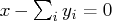$x - \sum_i y_i = 0$ does not constrain , since it must be nonnegative if all the 's are nonnegative. In this case, eliminate by subtracting this equation from all others containing . This is useful when the only other entry for is in the objective function. Perform this reduction if there is at most one other nonobjective coefficient. PRSLTYPE=0 reductions are also done.
3	All possible reductions are performed. PRSLTYPE=3 is the default.

Preprocessing is iterative. As variables are fixed and eliminated, and constraints are found to be redundant and they too are eliminated, and as variable bounds and constraint right-hand sides are tightened, the LP to be optimized is modified to reflect these changes. Another iteration of preprocessing of the modified LP may reveal more variables and constraints that can be eliminated.

PRINTLEVEL2=p

is used when you want to see PROC NETFLOW's progress to the optimum. PROC NETFLOW will produce a table on the SAS log. A row of the table is generated during each iteration and may consist of values of

the affine step complementarity
the complementarity of the solution for the next iteration
the total bound infeasibility $\sum_{i=1}^n {infeas}_{b i}$ (see the ${infeas}_b$ array in the section "Interior Point: Upper Bounds")
the total constraint infeasibility $\sum_{i=1}^m {infeas}_{c i}$ (see the ${infeas}_c$ array in the section "Interior Point Algorithmic Details")
the total dual infeasibility $\sum_{i=1}^n {infeas}_{d i}$ (see the ${infeas}_d$ array in the section "Interior Point Algorithmic Details")

As optimization progresses, the values in all columns should converge to zero. If you specify PRINTLEVEL2=2, all columns will appear in the table. If PRINTLEVEL2=1 is specified, only the affine step complementarity and the complementarity of the solution for the next iteration will appear. Some time is saved by not calculating the infeasibility values.

Interior Point Algorithm Options: Stopping Criteria

MAXITERB=m
IMAXITERB=m: specifies the maximum number of iterations of the interior point algorithm that can be performed. The default value for m is 100. One of the most remarkable aspects of the interior point algorithm is that for most problems, it usually needs to do a small number of iterations, no matter the size of the problem.
PDGAPTOL=p
RPDGAPTOL=p: specifies the primal-dual gap or duality gap tolerance. Duality gap is defined in the section "Interior Point Algorithmic Details". If the relative gap $({dualitygap}/(c^t x))$ between the primal and dual objectives is smaller than the value of the PDGAPTOL= option and both the primal and dual problems are feasible, then PROC NETFLOW stops optimization with a solution that is deemed optimal. Valid values for p are between 1.0E-12 and 1.0E-1. The default is 1.0E-7.
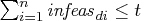
STOP_C=s: is used to determine whether optimization should stop. At the beginning of each iteration, if complementarity (the value of the Complem-ity column in the table produced when you specify PRINTLEVEL2=1 or PRINTLEVEL2=2) is $\le$ s, optimization will stop. This option is discussed in the section "Stopping Criteria".
STOP_DG=s: is used to determine whether optimization should stop. At the beginning of each iteration, if the duality gap (the value of the Duality_gap column in the table produced when you specify PRINTLEVEL2=1 or PRINTLEVEL2=2) is $\le$ s, optimization will stop. This option is discussed in the section "Stopping Criteria".
STOP_IB=s: is used to determine whether optimization should stop. At the beginning of each iteration, if total bound infeasibility $\sum_{i=1}^n {infeas}_{b i}$ (see the ${infeas}_b$ array in the section "Interior Point: Upper Bounds"; this value appears in the Tot_infeasb column in the table produced when you specify PRINTLEVEL2=1 or PRINTLEVEL2=2) is $\le$ s, optimization will stop. This option is discussed in the section "Stopping Criteria".
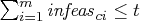
STOP_IC=s: is used to determine whether optimization should stop. At the beginning of each iteration, if total constraint infeasibility $\sum_{i=1}^m {infeas}_{c i}$ (see the ${infeas}_c$ array in the section "Interior Point Algorithmic Details"; this value appears in the Tot_infeasc column in the table produced when you specify PRINTLEVEL2=2) is $\le$ s, optimization will stop. This option is discussed in the section "Stopping Criteria".
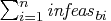
STOP_ID=s: is used to determine whether optimization should stop. At the beginning of each iteration, if total dual infeasibility $\sum_{i=1}^n {infeas}_{d i}$ (see the ${infeas}_d$ array in the section "Interior Point Algorithmic Details"; this value appears in the Tot_infeasd column in the table produced when you specify PRINTLEVEL2=2) is $\le$ s, optimization will stop. This option is discussed in the section "Stopping Criteria".
AND_STOP_C=s: is used to determine whether optimization should stop. At the beginning of each iteration, if complementarity (the value of the Complem-ity column in the table produced when you specify PRINTLEVEL2=1 or PRINTLEVEL2=2) is $\le$ s, and the conditions related to other AND_STOP parameters are also satisfied, optimization will stop. This option is discussed in the section "Stopping Criteria".
AND_STOP_DG=s: is used to determine whether optimization should stop. At the beginning of each iteration, if the duality gap (the value of the Duality_gap column in the table produced when you specify PRINTLEVEL2=1 or PRINTLEVEL2=2) is $\le$ s, and the conditions related to other AND_STOP parameters are also satisfied, optimization will stop. This option is discussed in the section "Stopping Criteria".
AND_STOP_IB=s: is used to determine whether optimization should stop. At the beginning of each iteration, if total bound infeasibility $\sum_{i=1}^n {infeas}_{b i}$ (see the ${infeas}_b$ array in the section "Interior Point: Upper Bounds"; this value appears in the Tot_infeasb column in the table produced when you specify PRINTLEVEL2=1 or PRINTLEVEL2=2) is $\le$ s, and the conditions related to other AND_STOP parameters are also satisfied, optimization will stop. This option is discussed in the section "Stopping Criteria".
AND_STOP_IC=s: is used to determine whether optimization should stop. At the beginning of each iteration, if total constraint infeasibility $\sum_{i=1}^m {infeas}_{c i}$ (see the ${infeas}_c$ array in the section "Interior Point Algorithmic Details"; this value appears in the Tot_infeasc column in the table produced when you specify PRINTLEVEL2=2) is $\le$ s, and the conditions related to other AND_STOP parameters are also satisfied, optimization will stop. This option is discussed in the section "Stopping Criteria".
AND_STOP_ID=s: is used to determine whether optimization should stop. At the beginning of each iteration, if total dual infeasibility $\sum_{i=1}^n {infeas}_{d i}$ (see the ${infeas}_d$ array in the section "Interior Point Algorithmic Details"; this value appears in the Tot_infeasd column in the table produced when you specify PRINTLEVEL2=2) is $\le$ s, and the conditions related to other AND_STOP parameters are also satisfied, optimization will stop. This option is discussed in the section "Stopping Criteria".
KEEPGOING_C=s: is used to determine whether optimization should stop. If a stopping condition is met, if complementarity (the value of the Complem-ity column in the table produced when you specify PRINTLEVEL2=1 or PRINTLEVEL2=2) is > s, optimization will continue. This option is discussed in the section "Stopping Criteria".
KEEPGOING_DG=s: is used to determine whether optimization should stop. If a stopping condition is met, if the duality gap (the value of the Duality_gap column in the table produced when you specify PRINTLEVEL2=1 or PRINTLEVEL2=2) is > s, optimization will continue. This option is discussed in the section "Stopping Criteria".
KEEPGOING_IB=s: is used to determine whether optimization should stop. If a stopping condition is met, if total bound infeasibility $\sum_{i=1}^n {infeas}_{b i}$ (see the ${infeas}_b$ array in the section "Interior Point: Upper Bounds"; this value appears in the Tot_infeasb column in the table produced when you specify PRINTLEVEL2=1 or PRINTLEVEL2=2) is > s, optimization will continue. This option is discussed in the section "Stopping Criteria".
KEEPGOING_IC=s: is used to determine whether optimization should stop. If a stopping condition is met, if total constraint infeasibility $\sum_{i=1}^m {infeas}_{c i}$ (see the ${infeas}_c$ array in the section "Interior Point Algorithmic Details"; this value appears in the Tot_infeasc column in the table produced when you specify PRINTLEVEL2=2) is > s, optimization will continue. This option is discussed in the section "Stopping Criteria".
KEEPGOING_ID=s: is used to determine whether optimization should stop. If a stopping condition is met, if total dual infeasibility $\sum_{i=1}^n {infeas}_{d i}$ (see the ${infeas}_d$ array in the section "Interior Point Algorithmic Details"; this value appears in the Tot_infeasd column in the table produced when you specify PRINTLEVEL2=2) is > s, optimization will continue. This option is discussed in the section "Stopping Criteria".
AND_KEEPGOING_C=s: is used to determine whether optimization should stop. If a stopping condition is met, if complementarity (the value of the Complem-ity column in the table produced when you specify PRINTLEVEL2=1 or PRINTLEVEL2=2) is > s, and the conditions related to other AND_KEEPGOING parameters are also satisfied, optimization will continue. This option is discussed in the section "Stopping Criteria".
AND_KEEPGOING_DG=s: is used to determine whether optimization should stop. If a stopping condition is met, if the duality gap (the value of the Duality_gap column in the table produced when you specify PRINTLEVEL2=1 or PRINTLEVEL2=2) is > s, and the conditions related to other AND_KEEPGOING parameters are also satisfied, optimization will continue. This option is discussed in the section "Stopping Criteria".
AND_KEEPGOING_IB=s: is used to determine whether optimization should stop. If a stopping condition is met, if total bound infeasibility $\sum_{i=1}^n {infeas}_{b i}$ (see the ${infeas}_b$ array in the section "Interior Point: Upper Bounds"; this value appears in the Tot_infeasb column in the table produced when you specify PRINTLEVEL2=2) is > s, and the conditions related to other AND_KEEPGOING parameters are also satisfied, optimization will continue. This option is discussed in the section "Stopping Criteria".
AND_KEEPGOING_IC=s: is used to determine whether optimization should stop. If a stopping condition is met, if total constraint infeasibility $\sum_{i=1}^m {infeas}_{c i}$ (see the ${infeas}_c$ array in the section "Interior Point Algorithmic Details"; this value appears in the Tot_infeasc column in the table produced when you specify PRINTLEVEL2=2) is > s, and the conditions related to other AND_KEEPGOING parameters are also satisfied, optimization will continue. This option is discussed in the section "Stopping Criteria".
AND_KEEPGOING_ID=s: is used to determine whether optimization should stop. If a stopping condition is met, if total dual infeasibility $\sum_{i=1}^n {infeas}_{d i}$ (see the ${infeas}_d$ array in the section "Interior Point Algorithmic Details"; this value appears in the Tot_infeasd column in the table produced when you specify PRINTLEVEL2=2) is > s, and the conditions related to other AND_KEEPGOING parameters are also satisfied, optimization will continue. This option is discussed in the section "Stopping Criteria".

Top of Page