Previous Page

|

Next Page

Example 7.3: Solving NLP Problems with Range Constraints

Often there are constraints with both lower and upper bounds, i.e., . These constraints are called range constraints . The IPNLP solver can handle range constraints in an efficient way. Consider the following NLP problem:

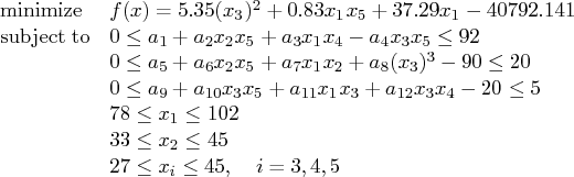
where the values of the parameters , are shown in Table 7.2.

1	85.334407	5	80.51249	9	0.0047026
2	0.0056858	6	0.0071317	10	0.0012547
3	0.0006262	7	0.0029955	11	0.0019085
4	0.0022053	8	0.0021813	12	0.0019085

The initial point used is . You can call the IPNLP solver within PROC OPTMODEL to solve this problem by writing the following SAS code:

    proc optmodel;
       number l {1..5} = [78 33 27 27 27];
       number u {1..5} = [102 45 45 45 45];
    
       number a {1..12} = 
          [85.334407 0.0056858 0.0006262 0.0022053
          80.51249 0.0071317 0.0029955 0.0021813
          9.300961 0.0047026 0.0012547 0.0019085];
    
       var x {j in 1..5} >= l[j] <= u[j];
    
       minimize obj = 5.35*x[3]^2 + 0.83*x[1]*x[5] + 37.29*x[1] 
                      - 40792.141;
    
       con constr1: 
          0 <= a[1] + a[2]*x[2]*x[5] + a[3]*x[1]*x[4] - 
             a[4]*x[3]*x[5] <= 92;
       con constr2: 
          0 <= a[5] + a[6]*x[2]*x[5] + a[7]*x[1]*x[2] + 
             a[8]*x[3]^2 - 90 <= 20;
       con constr3: 
          0 <= a[9] + a[10]*x[3]*x[5] + a[11]*x[1]*x[3] + 
             a[12]*x[3]*x[4] -20 <= 5;
    
       x[1] = 78;
       x[2] = 33;
       x[3] = 27;
       x[4] = 27;
       x[5] = 27;
    
       solve with ipnlp;
       print x;
    quit;
 

The summaries and the optimal solution are shown in Output 7.3.1.